Introduction

“You can’t prove a hypothesis; you can only improve or disprove it.” – Christopher Monckton

Every day we find ourselves testing new ideas, finding the fastest route to the office, the quickest way to finish our work, or simply finding a better way to do something we love. The critical question, then, is whether our idea is significantly better than what we tried previously.

These ideas that we come up with on such a regular basis – that’s essentially what a hypothesis is. And testing these ideas to figure out which one works and which one is best left behind, is called hypothesis testing.

Hypothesis testing is one of the most fascinating things we do as data scientists. No idea is off-limits at this stage of our project. I have personally seen so many insights coming out of hypothesis testing – insights most of us would have missed if not for this stage!

One of the most popular ways to test a hypothesis is a concept called the t-test. There are different types of t-tests, as we’ll soon see, and each one has its own unique application. If you’re an aspiring data scientist, you should be aware of what a t-test is and when you can leverage it.

So in this article, we will learn about the various nuances of a t-test and then look at the three different t-test types. The icing on the cake? We will implement each type of t-test in R to visualize how they work in practical scenarios. Let’s get going!

Note: You should go through the below article if you need to brush up on your hypothesis testing concepts:

• Guide to Master Hypothesis Testing in Statistics

 

Table of Contents

1. When should we Perform a t-test?
2. Assumptions for Performing a t-test
3. Types of t-tests (with Solved Examples in R)
   • One-Sample t-test
   • Independent Two-Sample t-test
   • Paired Sample t-test

 

When should we Perform a t-test?

Let’s first understand where a t-test can be used before we dive into its different types and their implementations. I strongly believe the best way to learn a concept is by visualizing it through an example. So let’s take a simple example to see where a t-test comes in handy.

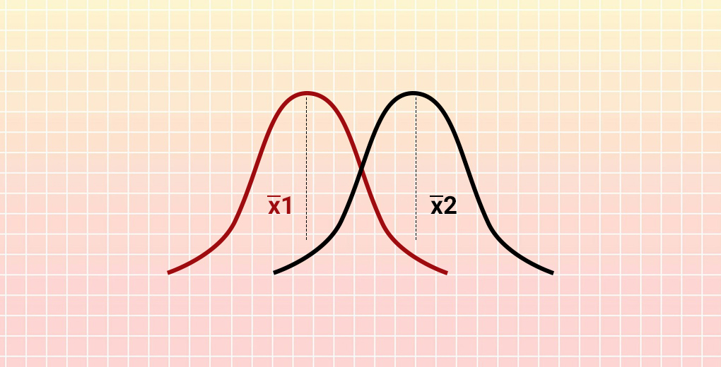
Consider a telecom company that has two service centers in the city. The company wants to find whether the average time required to service a customer is the same in both stores.

The company measures the average time taken by 50 random customers in each store. Store A takes 22 minutes while Store B averages 25 minutes. Can we say that Store A is more efficient than Store B in terms of customer service?

It does seem that way, doesn’t it? However, we have only looked at 50 random customers out of the many people who visit the stores. Simply looking at the average sample time might not be representative of all the customers who visit both the stores.

This is where the t-test comes into play. It helps us understand if the difference between two sample means is actually real or simply due to chance.

 

Assumptions for Performing a t-test

There are certain assumptions we need to heed before performing a t-test:

1. The data should follow a continuous or ordinal scale (the IQ test scores of students, for example)
2. The observations in the data should be randomly selected
3. The data should resemble a bell-shaped curve when we plot it, i.e., it should be normally distributed. You can refer to this article to get a better understanding of the normal distribution
4. Large sample size should be taken for the data to approach a normal distribution (although t-test is essential for small samples as their distributions are non-normal)
5. Variances among the groups should be equal (for independent two-sample t-test)

So what are the different types of t-tests? When should we perform each type? We’ll answer these questions in the next section and see how we can perform each t-test type in R.

 

Types of t-tests (with Solved Examples in R)

There are three types of t-tests we can perform based on the data at hand:

• One sample t-test
• Independent two-sample t-test
• Paired sample t-test

In this section, we will look at each of these types in detail. I have also provided the R code for each t-test type so you can follow along as we implement them. It’s a great way to learn and see how useful these t-tests are!

 

One-Sample t-test

In a one-sample t-test, we compare the average (or mean) of one group against the set average (or mean). This set average can be any theoretical value (or it can be the population mean).

Consider the following example – A research scholar wants to determine if the average eating time for a (standard size) burger differs from a set value. Let’s say this value is 10 minutes. How do you think the research scholar can go about determining this?

He/she can broadly follow the below steps:

• Select a group of people
• Record the individual eating time of a standard size burger
• Calculate the average eating time for the group
• Finally, compare that average value with the set value of 10

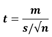
That, in a nutshell, is how we can perform a one-sample t-test. Here’s the formula to calculate this:

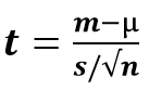
where,

• t = t-statistic
• m = mean of the group
• µ = theoretical value or population mean
• s = standard deviation of the group
• n = group size or sample size

Note: As mentioned earlier in the assumptions that large sample size should be taken for the data to approach a normal distribution. (Although t-test is essential for small samples as their distributions are non-normal).

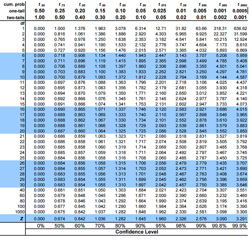
Once we have calculated the t-statistic value, the next task is to compare it with the critical value of the t-test. We can find this in the below t-test table against the degree of freedom (n-1) and the level of significance:

This method helps us check whether the difference between the means is statistically significant or not. Let’s further solidify our understanding of a one-sample t-test by performing it in R.

 

Implementing the One-Sample t-test in R

A mobile manufacturing company has taken a sample of mobiles of the same model from the previous month’s data. They want to check whether the average screen size of the sample differs from the desired length of 10 cm. You can download the data here.

Step 1: First, import the data.

Step 2: Validate it for correctness in R:

Output:

#Count of Rows and columns
[1] 1000    1
> #View top 10 rows of the dataset
   Screen_size.in.cm.
1           10.006692
2           10.081624
3           10.072873
4            9.954496
5            9.994093
6            9.952208
7            9.947936
8            9.988184
9            9.993365
10          10.016660

Step 3: Remember the assumptions we discussed earlier? We need to check them:

We get the below Q-Q plot:

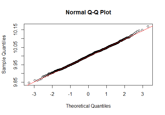
Almost all the values lie on the red line. We can confidently say that the data follows a normal distribution.

Step 4: Conduct a one-sample t-test:

Output:

	One Sample t-test

data:  data$Screen_size.in.cm.
t = -0.39548, df = 999, p-value = 0.6926
alternative hypothesis: true mean is not equal to 10
95 percent confidence interval:
  9.996361 10.002418
sample estimates:
mean of x 
  9.99939

The t-statistic comes out to be -0.39548. Note that we can treat negative values as their positive counterpart here. Now, refer to the table mentioned earlier for the t-critical value. The degree of freedom here is 999 and the confidence interval is 95%.

The t-critical value is 1.962. Since the t-statistic is less than the t-critical value, we fail to reject the null hypothesis and can conclude that the average screen size of the sample does not differ from 10 cm.

We can also verify this from the p-value, which is greater than 0.05. Therefore, we fail to reject the null hypothesis at a 95% confidence interval.

 

Independent Two-Sample t-test

The two-sample t-test is used to compare the means of two different samples.

Let’s say we want to compare the average height of the male employees to the average height of the females. Of course, the number of males and females should be equal for this comparison. This is where a two-sample t-test is used.

Here’s the formula to calculate the t-statistic for a two-sample t-test:

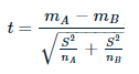
where,

• m_A and m_B are the means of two different samples
• n_A and n_B are the sample sizes
• S² is an estimator of the common variance of two samples, such as:

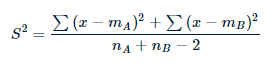
Here, the degree of freedom is n_A + n_B – 2.

We will follow the same logic we saw in a one-sample t-test to check if the average of one group is significantly different from another group. That’s right – we will compare the calculated t-statistic with the t-critical value.

Let’s take an example of an independent two-sample t-test and solve it in R.

 

Implementing the Two-Sample t-test in R

For this section, we will work with data about two samples of the various models of a mobile phone. We want to check whether the mean screen size of sample 1 differs from the mean screen size of sample 2. You can download the data here.

Step 1: Again, first import the data.

Step 2: Validate it for correctness in R:

Step 3:  We need to check the assumptions as we did above. I will leave that exercise up to you now.

Also, in this case, we will check the homogeneity of variance:

Output:

 #Homogeneity of variance
> var(data$screensize_sample1)
[1] 0.00238283
> var(data$screensize_sample2)
[1] 0.002353585

Great, the variances are equal. We can move ahead.

Step 4: Conduct the independent two-sample t-test:

Note: Rewrite the above code with “var.equal = F” if you get unequal or unknown variances. This will be a case of Welch’s t-test which is used to compare the means of two samples with unequal variances.

Output:

Two Sample t-test

data: data$screensize_sample1 and data$screensize_sample2
t = 1.3072, df = 1998, p-value = 0.1913
alternative hypothesis: true difference in means is not equal to 0
95 percent confidence interval:
-0.001423145 0.007113085
sample estimates:
mean of x mean of y 
10.000976 9.998131

What can you infer from the above output? We can confirm that the t-statistic is again less than the t-critical value so we fail to reject the null hypothesis. Hence, we can conclude that there is no difference between the mean screen size of both samples.

We can verify this again using the p-value. It comes out to be greater than 0.05, therefore we fail to reject the null hypothesis at a 95% confidence interval. There is no difference between the mean of the two samples.

 

Paired Sample t-test

The paired sample t-test is quite intriguing. Here, we measure one group at two different times. We compare separate means for a group at two different times or under two different conditions. Confused? Let me explain.

A certain manager realized that the productivity level of his employees was trending significantly downwards. This manager decided to conduct a training program for all his employees with the aim of increasing their productivity levels.

How will the manager measure if the productivity levels increased? It’s simple – just compare the productivity level of the employees before versus after the training program.

Here, we are comparing the same sample (the employees) at two different times (before and after the training). This is an example of a paired t-test. The formula to calculate the t-statistic for a paired t-test is:

where,

• t = t-statistic
• m = mean of the group
• µ = theoretical value or population mean
• s = standard deviation of the group
• n = group size or sample size

We can take the degree of freedom in this test as n – 1 since only one group is involved. Now, let’s solve an example in R.

 

Implementing the Paired t-test in R

The manager of a tyre manufacturing company wants to compare the rubber material for two lots of tyres. One way to do this – check the difference between average kilometers covered by one lot of tyres until they wear out.

You can download the data from here. Let’s do this!

Step 1: First, import the data.

Step 2: Validate it for correctness in R:

Step 3: We now check the assumptions just as we did in a one-sample t-test. Again, I will leave this to you.

Step 4: Conduct the paired t-test:

Output:

Paired t-test

data: data$tyre_1 and data$tyre_2
t = -5.2662, df = 24, p-value = 2.121e-05
alternative hypothesis: true difference in means is not equal to 0
95 percent confidence interval:
-2201.6929 -961.8515
sample estimates:
mean of the differences 
-1581.772

You must be a pro at deciphering this output by now! The p-value is less than 0.05. We can reject the null hypothesis at a 95% confidence interval and conclude that there is a significant difference between the means of tyres before and after the rubber material replacement.

The negative mean in the difference depicts that the average kilometers covered by tyre 2 are more than the average kilometers covered by tyre 1.

 

End Notes

In this article, we learned about the concept of t-test, its assumptions, and also the three different types of t-tests with their implementations in R. The t-test has both statistical significance as well as practical applications in the real world.

If you are new to statistics, want to cover your basics, and also want to get a start in data science, I recommend taking the Introduction to Data Science course. It gives you a comprehensive overview of both descriptive and inferential statistics before diving into data science techniques.

Did you find this article useful? Can you think of any other applications of the t-test? Let me know in the comments section below and we can come up with more ideas!