Introduction

What is one of the most important and core concepts of statistics that enables us to do predictive modeling, and yet it often confuses aspiring data scientists? Yes, I’m talking about the central limit theorem.

It is a powerful statistical concept that every data scientist MUST know. Now, why is that?

Well, the central limit theorem (CLT) is at the heart of hypothesis testing – a critical component of the data science lifecycle. That’s right, the idea that lets us explore the vast possibilities of the data we are given springs from CLT. It’s actually a simple notion to understand, yet most data scientists flounder at this question during interviews.

We will understand the concept of Central Limit Theorem (CLT) in this article. We’ll see why it’s important, where it’s used and then learn how to apply it in R.

I recommend going through the below article if you need a quick refresher on distribution and its various types:

• 6 Common Probability Distributions every data science professional should know

 

Table of Contents

1. What is the Central Limit Theorem (CLT)?
2. Significance of the Central Limit Theorem
   • Statistical Significance
   • Practical Applications
3. Assumptions Behind the Central Limit Theorem
4. Implementing the Central Limit Theorem in R

 

What is the Central Limit Theorem (CLT)?

Let’s understand the central limit theorem with the help of an example. This will help you intuitively grasp how CLT works underneath.

Consider that there are 15 sections in the science department of a university and each section hosts around 100 students. Our task is to calculate the average weight of students in the science department. Sounds simple, right?

The approach I get from aspiring data scientists is to simply calculate the average:

• First, measure the weights of all the students in the science department
• Add all the weights
• Finally, divide the total sum of weights with a total number of students to get the average

But what if the size of the data is humongous? Does this approach make sense? Not really – measuring the weight of all the students will be a very tiresome and long process. So, what can we do instead? Let’s look at an alternate approach.

• First, draw groups of students at random from the class. We will call this a sample. We’ll draw multiple samples, each consisting of 30 students.

Source: http://www.123rf.com

• Calculate the individual mean of these samples
• Calculate the mean of these sample means
• This value will give us the approximate mean weight of the students in the science department
• Additionally, the histogram of the sample mean weights of students will resemble a bell curve (or normal distribution)

This, in a nutshell, is what the central limit theorem is all about. If you take your learning through videos, check out the below introduction to the central limit theorem. This is part of the comprehensive statistics module in the ‘Introduction to Data Science’ course:

 

Formally Defining the Central Limit Theorem

Let’s put a formal definition to CLT:

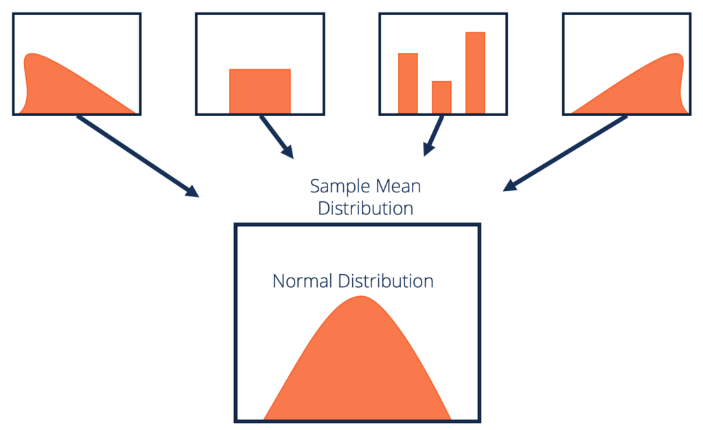
Given a dataset with unknown distribution (it could be uniform, binomial or completely random), the sample means will approximate the normal distribution.

These samples should be sufficient in size. The distribution of sample means, calculated from repeated sampling, will tend to normality as the size of your samples gets larger.

Source: corporatefinanceinstitute.com

The central limit theorem has a wide variety of applications in many fields. Let us look at them in the next section.

 

Significance of the Central Limit Theorem

The central limit theorem has both statistical significance as well as practical applications. Isn’t that the sweet spot we aim for when we’re learning a new concept?

We’ll look at both aspects to gauge where we can use them.

 

 Statistical Significance of CLT

• Analyzing data involves statistical methods like hypothesis testing and constructing confidence intervals. These methods assume that the population is normally distributed. In the case of unknown or non-normal distributions, we treat the sampling distribution as normal according to the central limit theorem
• If we increase the samples drawn from the population, the standard deviation of sample means will decrease. This helps us estimate the population mean much more accurately
• Also, the sample mean can be used to create the range of values known as a confidence interval (that is likely to consist of the population mean)

 

 Practical Applications of CLT

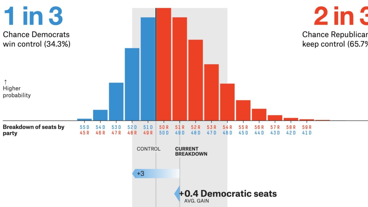
Source: projects.fivethirtyeight.com

• Political/election polls are prime CLT applications. These polls estimate the percentage of people who support a particular candidate. You might have seen these results on news channels that come with confidence intervals. The central limit theorem helps calculate that
• Confidence interval, an application of CLT, is used to calculate the mean family income for a particular region

The central limit theorem has many applications in different fields. Can you think of more examples? Let me know in the comments section below the article – I will include them here.

 

Assumptions Behind the Central Limit Theorem

Before we dive into the implementation of the central limit theorem, it’s important to understand the assumptions behind this technique:

1. The data must follow the randomization condition. It must be sampled randomly
2. Samples should be independent of each other. One sample should not influence the other samples
3. Sample size should be not more than 10% of the population when sampling is done without replacement
4. The sample size should be sufficiently large. Now, how we will figure out how large this size should be? Well, it depends on the population. When the population is skewed or asymmetric, the sample size should be large. If the population is symmetric, then we can draw small samples as well

In general, a sample size of 30 is considered sufficient when the population is symmetric.

The mean of the sample means is denoted as:

µ _X̄ = µ

where,

• µ _X̄ = Mean of the sample means
• µ= Population mean

And, the standard deviation of the sample mean is denoted as:

σ _X̄ = σ/sqrt(n)

where,

• σ _X̄ = Standard deviation of the sample mean
• σ = Population standard deviation
• n = sample size

And that’s it for the concept behind central limit theorem. Time to fire up RStudio and dig into CLT’s implementation!

 

Implementing the Central Limit Theorem in R

Excited to see how we can code the central limit theorem in R? Let’s dig in then.

 

Understanding the Problem Statement

A pipe manufacturing organization produces different kinds of pipes. We are given the monthly data of the wall thickness of certain types of pipes. You can download the data here.

The organization wants to analyze the data by performing hypothesis testing and constructing confidence intervals to implement some strategies in the future. The challenge is that the distribution of the data is not normal.

Note: This analysis works on a few assumptions and one of them is that the data should be normally distributed.

 

Solution Methodology

The central limit theorem will help us get around the problem of this data where the population is not normal. Therefore, we will simulate the central limit theorem on the given dataset in R step-by-step. So, let’s get started.

 

Import the CSV Dataset and Validate it

First, import the CSV file in R and then validate the data for correctness:

Output:

#Count of Rows and columns
9000 1

#View top 10 rows of the dataset
   Wall.Thickness
1        12.35487
2        12.61742
3        12.36972
4        13.22335
5        13.15919
6        12.67549
7        12.36131
8        12.44468
9        12.62977
10       12.90381

#View last 10 rows of the dataset
     Wall.Thickness
8991       12.65444
8992       12.80744
8993       12.93295
8994       12.33271
8995       12.43856
8996       12.99532
8997       13.06003
8998       12.79500
8999       12.77742
9000       13.01416

Next, calculate the population mean and plot all the observations of the data:

Output:

#Calculate the population mean
[1] 12.80205

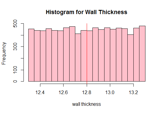
See the red vertical line above? That’s the population mean. We can also see from the above plot that the population is not normal, right? Therefore, we need to draw sufficient samples of different sizes and compute their means (known as sample means). We will then plot those sample means to get a normal distribution.

In our example, we will draw sufficient samples of size 10, calculate their means, and plot them in R. I know that the minimum sample size taken should be 30 but let’s just see what happens when we draw 10:

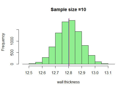
Now, we know that we’ll get a very nice bell-shaped curve as the sample sizes increase. Let us now increase our sample size and see what we get:

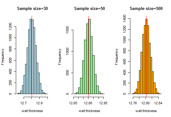
Here, we get a good bell-shaped curve and the sampling distribution approaches normal distribution as the sample sizes increase. Therefore, we can consider the sampling distributions as normal and the pipe manufacturing organization can use these distributions for further analysis.

You can also play around by taking different sample sizes and drawing a different number of samples. Let me know how it works out for you!

 

End Notes

Central limit theorem is quite an important concept in statistics, and consequently data science. I cannot stress enough on how critical it is that you brush up on your statistics knowledge before getting into data science or even sitting for a data science interview.

I recommend taking the Introduction to Data Science course – it’s a comprehensive look at statistics before introducing data science.

If you have any doubts or feedback, do let me know in the comments section below.