A Hands-On Introduction to Deep Q-Learning using OpenAI Gym in Python

Ankit Choudhary 27 Apr, 2020 • 10 min read

Introduction

I have always been fascinated with games. The seemingly infinite options available to perform an action under a tight timeline – it’s a thrilling experience. There’s nothing quite like it.

So when I read about the incredible algorithms DeepMind was coming up with (like AlphaGo and AlphaStar), I was hooked. I wanted to learn how to make these systems on my own machine. And that led me into the world of deep reinforcement learning (Deep RL).

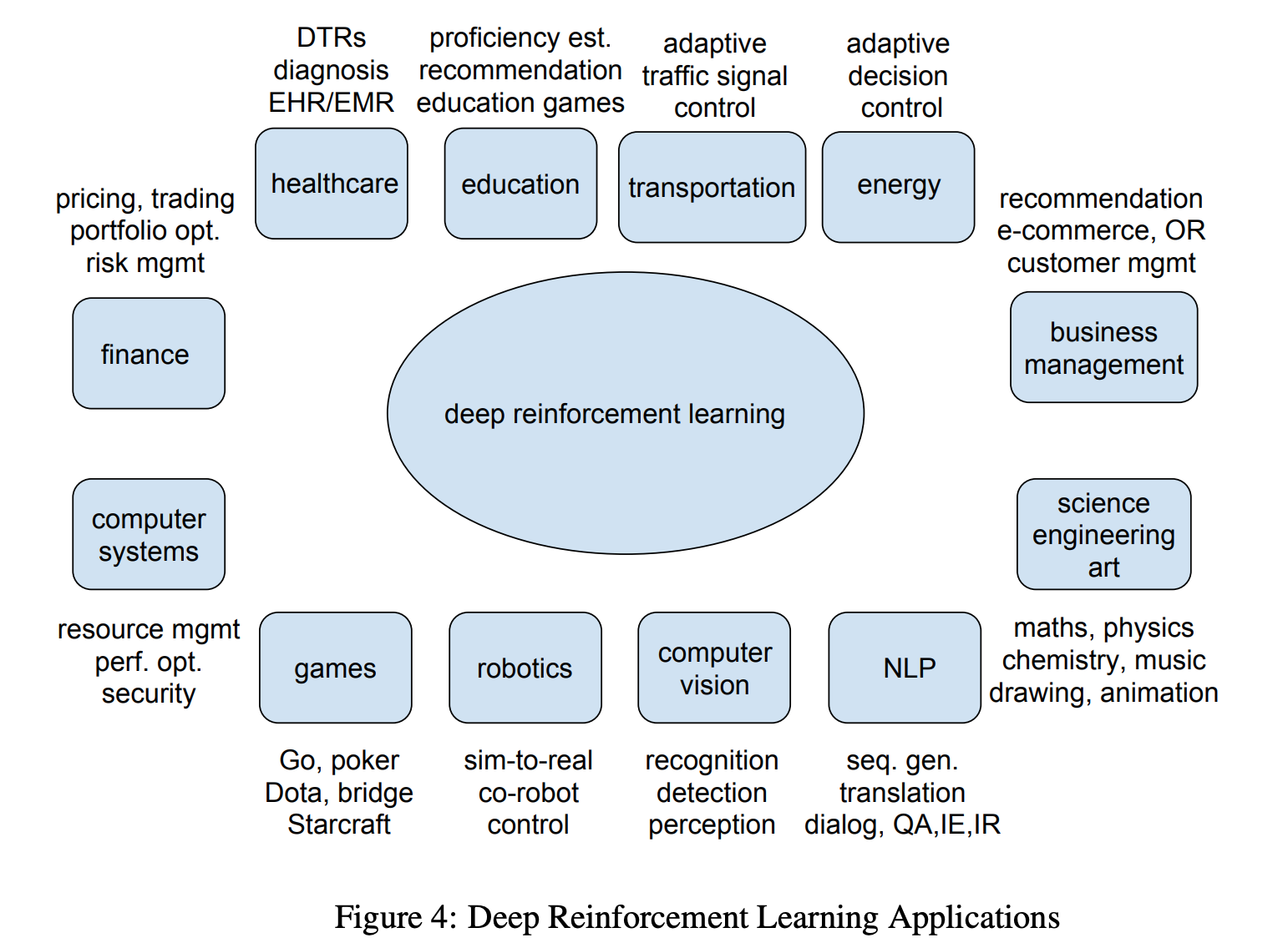
Deep RL is relevant even if you’re not into gaming. Just check out the sheer variety of functions currently using Deep RL for research:

What about industry-ready applications? Well, here are two of the most commonly cited Deep RL use cases:

Google’s Cloud AutoML
Facebook’s Horizon Platform

The scope of Deep RL is IMMENSE. This is a great time to enter into this field and make a career out of it.

In this article, I aim to help you take your first steps into the world of deep reinforcement learning. We’ll use one of the most popular algorithms in RL, deep Q-learning, to understand how deep RL works. And the icing on the cake? We will implement all our learning in an awesome case study using Python.

The Road to Q-Learning

There are certain concepts you should be aware of before wading into the depths of deep reinforcement learning. Don’t worry, I’ve got you covered.

I have previously written various articles on the nuts and bolts of reinforcement learning to introduce concepts like multi-armed bandit, dynamic programming, Monte Carlo learning and temporal differencing. I recommend going through these guides in the below sequence:

These articles are good enough for getting a detailed overview of basic RL from the beginning.

However, note that the articles linked above are in no way prerequisites for the reader to understand Deep Q-Learning. We will do a quick recap of the basic RL concepts before exploring what is deep Q-Learning and its implementation details.

RL Agent-Environment

A reinforcement learning task is about training an agent which interacts with its environment. The agent arrives at different scenarios known as states by performing actions. Actions lead to rewards which could be positive and negative.

The agent has only one purpose here – to maximize its total reward across an episode. This episode is anything and everything that happens between the first state and the last or terminal state within the environment. We reinforce the agent to learn to perform the best actions by experience. This is the strategy or policy.

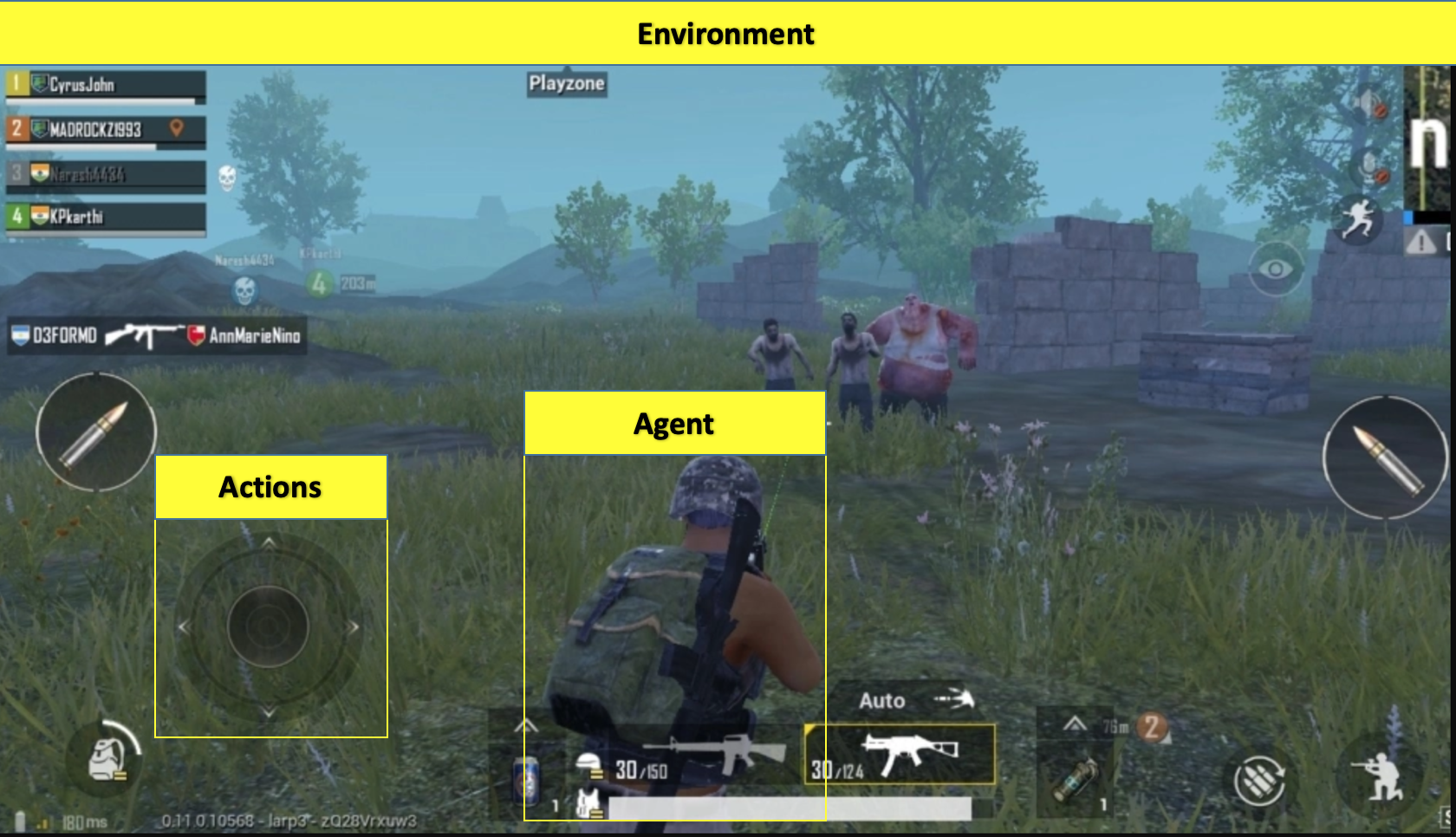
Let’s take an example of the ultra-popular PubG game:

The soldier is the agent here interacting with the environment
The states are exactly what we see on the screen
An episode is a complete game
The actions are moving forward, backward, left, right, jump, duck, shoot, etc.
Rewards are defined on the basis of the outcome of these actions. If the soldier is able to kill an enemy, that calls for a positive reward while getting shot by an enemy is a negative reward

Now, in order to kill that enemy or get a positive reward, there is a sequence of actions required. This is where the concept of delayed or postponed reward comes into play. The crux of RL is learning to perform these sequences and maximizing the reward.

Markov Decision Process (MDP)

An important point to note – each state within an environment is a consequence of its previous state which in turn is a result of its previous state. However, storing all this information, even for environments with short episodes, will become readily infeasible.

To resolve this, we assume that each state follows a Markov property, i.e., each state depends solely on the previous state and the transition from that state to the current state. Check out the below maze to better understand the intuition behind how this works:

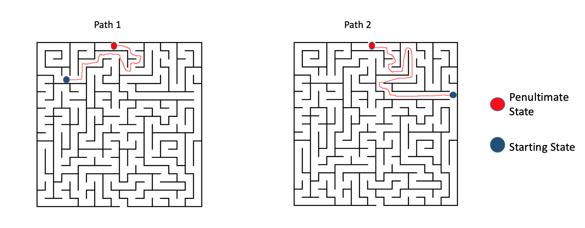
Now, there are 2 scenarios with 2 different starting points and the agent traverses different paths to reach the same penultimate state. Now it doesn’t matter what path the agent takes to reach the red state. The next step to exit the maze and reach the last state is by going right. Clearly, we only needed the information on the red/penultimate state to find out the next best action which is exactly what the Markov property implies.

Q Learning

Let’s say we know the expected reward of each action at every step. This would essentially be like a cheat sheet for the agent! Our agent will know exactly which action to perform.

It will perform the sequence of actions that will eventually generate the maximum total reward. This total reward is also called the Q-value and we will formalise our strategy as:

The above equation states that the Q-value yielded from being at state s and performing action a is the immediate reward r(s,a) plus the highest Q-value possible from the next state s’. Gamma here is the discount factor which controls the contribution of rewards further in the future.

Q(s’,a) again depends on Q(s”,a) which will then have a coefficient of gamma squared. So, the Q-value depends on Q-values of future states as shown here:

Adjusting the value of gamma will diminish or increase the contribution of future rewards.

Since this is a recursive equation, we can start with making arbitrary assumptions for all q-values. With experience, it will converge to the optimal policy. In practical situations, this is implemented as an update:

where alpha is the learning rate or step size. This simply determines to what extent newly acquired information overrides old information.

Why ‘Deep’ Q-Learning?

Q-learning is a simple yet quite powerful algorithm to create a cheat sheet for our agent. This helps the agent figure out exactly which action to perform.

But what if this cheatsheet is too long? Imagine an environment with 10,000 states and 1,000 actions per state. This would create a table of 10 million cells. Things will quickly get out of control!

It is pretty clear that we can’t infer the Q-value of new states from already explored states. This presents two problems:

First, the amount of memory required to save and update that table would increase as the number of states increases
Second, the amount of time required to explore each state to create the required Q-table would be unrealistic

Here’s a thought – what if we approximate these Q-values with machine learning models such as a neural network? Well, this was the idea behind DeepMind’s algorithm that led to its acquisition by Google for 500 million dollars!

Deep Q-Networks

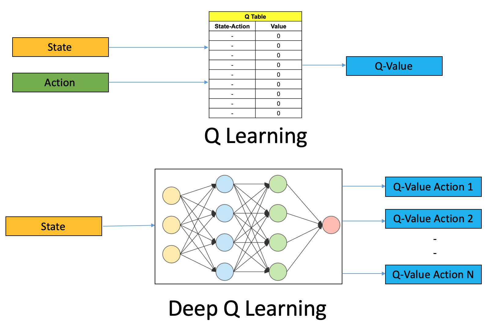
In deep Q-learning, we use a neural network to approximate the Q-value function. The state is given as the input and the Q-value of all possible actions is generated as the output. The comparison between Q-learning & deep Q-learning is wonderfully illustrated below:

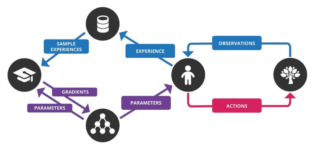
So, what are the steps involved in reinforcement learning using deep Q-learning networks (DQNs)?

All the past experience is stored by the user in memory
The next action is determined by the maximum output of the Q-network
The loss function here is mean squared error of the predicted Q-value and the target Q-value – Q*. This is basically a regression problem. However, we do not know the target or actual value here as we are dealing with a reinforcement learning problem. Going back to the Q-value update equation derived fromthe Bellman equation. we have:

The section in green represents the target. We can argue that it is predicting its own value, but since R is the unbiased true reward, the network is going to update its gradient using backpropagation to finally converge.

Challenges in Deep RL as Compared to Deep Learning

So far, this all looks great. We understood how neural networks can help the agent learn the best actions. However, there is a challenge when we compare deep RL to deep learning (DL):

Non-stationary or unstable target: Let us go back to the pseudocode for deep Q-learning:

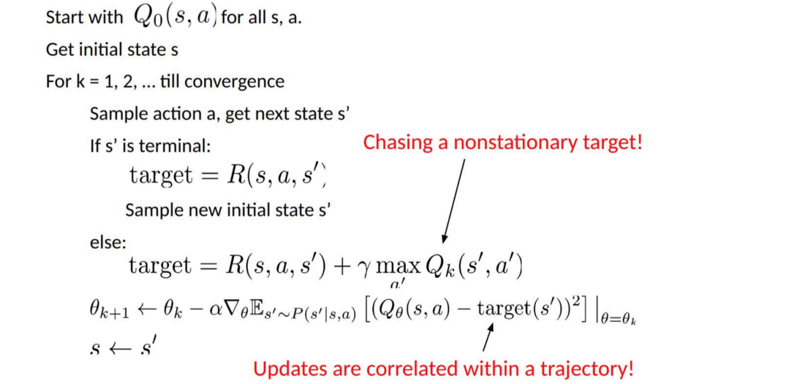
As you can see in the above code, the target is continuously changing with each iteration. In deep learning, the target variable does not change and hence the training is stable, which is just not true for RL.

To summarise, we often depend on the policy or value functions in reinforcement learning to sample actions. However, this is frequently changing as we continuously learn what to explore. As we play out the game, we get to know more about the ground truth values of states and actions and hence, the output is also changing.

So, we try to learn to map for a constantly changing input and output. But then what is the solution?

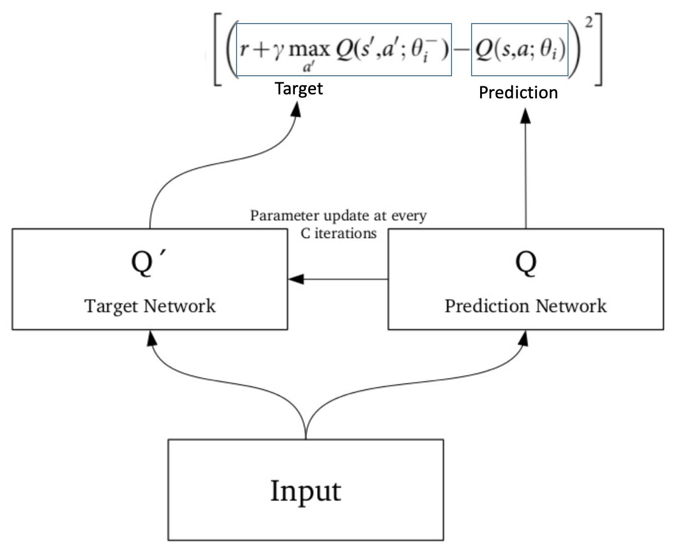
1. Target Network

Since the same network is calculating the predicted value and the target value, there could be a lot of divergence between these two. So, instead of using 1one neural network for learning, we can use two.

We could use a separate network to estimate the target. This target network has the same architecture as the function approximator but with frozen parameters. For every C iterations (a hyperparameter), the parameters from the prediction network are copied to the target network. This leads to more stable training because it keeps the target function fixed (for a while):

2. Experience Replay

To perform experience replay, we store the agent’s experiences – $e_{t} = (s_{t}, a_{t}, r_{t}, s_{t + 1})$

What does the above statement mean? Instead of running Q-learning on state/action pairs as they occur during simulation or the actual experience, the system stores the data discovered for [state, action, reward, next_state] – in a large table.

Let’s understand this using an example.

Suppose we are trying to build a video game bot where each frame of the game represents a different state. During training, we could sample a random batch of 64 frames from the last 100,000 frames to train our network. This would get us a subset within which the correlation amongst the samples is low and will also provide better sampling efficiency.

Putting it all Together

The concepts we have learned so far? They all combine to make the deep Q-learning algorithm that was used to achive human-level level performance in Atari games (using just the video frames of the game).

I have listed the steps involved in a deep Q-network (DQN) below:

Preprocess and feed the game screen (state s) to our DQN, which will return the Q-values of all possible actions in the state
Select an action using the epsilon-greedy policy. With the probability epsilon, we select a random action a and with probability 1-epsilon, we select an action that has a maximum Q-value, such as a = argmax(Q(s,a,w))
Perform this action in a state s and move to a new state s’ to receive a reward. This state s’ is the preprocessed image of the next game screen. We store this transition in our replay buffer as <s,a,r,s’>
Next, sample some random batches of transitions from the replay buffer and calculate the loss
It is known that: which is just the squared difference between target Q and predicted Q
Perform gradient descent with respect to our actual network parameters in order to minimize this loss
After every C iterations, copy our actual network weights to the target network weights
Repeat these steps for M number of episodes

Implementing Deep Q-Learning in Python using Keras & OpenAI Gym

Alright, so we have a solid grasp on the theoretical aspects of deep Q-learning. How about seeing it in action now? That’s right – let’s fire up our Python notebooks!

We will make an agent that can play a game called CartPole. We can also use an Atari game but training an agent to play that takes a while (from a few hours to a day). The idea behind our approach will remain the same so you can try this on an Atari game on your machine.

CartPole is one of the simplest environments in the OpenAI gym (a game simulator). As you can see in the above animation, the goal of CartPole is to balance a pole that’s connected with one joint on top of a moving cart.

Instead of pixel information, there are four kinds of information given by the state (such as the angle of the pole and position of the cart). An agent can move the cart by performing a series of actions of 0 or 1, pushing the cart left or right.

We will use the keras-rl library here which lets us implement deep Q-learning out of the box.

Step 1: Install keras-rl library

From the terminal, run the following code block:

git clone https://github.com/matthiasplappert/keras-rl.git
cd keras-rl
python setup.py install

Step 2: Install dependencies for the CartPole environment

Assuming you have pip installed, you need to install the following libraries:

pip install h5py
pip install gym

Step 3: Let’s get started!

First, we have to import the necessary modules:

import numpy as np
import gym

from keras.models import Sequential
from keras.layers import Dense, Activation, Flatten
from keras.optimizers import Adam

from rl.agents.dqn import DQNAgent
from rl.policy import EpsGreedyQPolicy
from rl.memory import SequentialMemory

Then, set the relevant variables:

ENV_NAME = 'CartPole-v0'

# Get the environment and extract the number of actions available in the Cartpole problem
env = gym.make(ENV_NAME)
np.random.seed(123)
env.seed(123)
nb_actions = env.action_space.n

Next, we will build a very simple single hidden layer neural network model:

model = Sequential()
model.add(Flatten(input_shape=(1,) + env.observation_space.shape))
model.add(Dense(16))
model.add(Activation('relu'))
model.add(Dense(nb_actions))
model.add(Activation('linear'))
print(model.summary())

Now, configure and compile our agent. We will set our policy as Epsilon Greedy and our memory as Sequential Memory because we want to store the result of actions we performed and the rewards we get for each action.

policy = EpsGreedyQPolicy()
memory = SequentialMemory(limit=50000, window_length=1)
dqn = DQNAgent(model=model, nb_actions=nb_actions, memory=memory, nb_steps_warmup=10,
target_model_update=1e-2, policy=policy)
dqn.compile(Adam(lr=1e-3), metrics=['mae'])

# Okay, now it's time to learn something! We visualize the training here for show, but this slows down training quite a lot. 
dqn.fit(env, nb_steps=5000, visualize=True, verbose=2)

Test our reinforcement learning model:

dqn.test(env, nb_episodes=5, visualize=True)

This will be the output of our model:

Not bad! Congratulations on building your very first deep Q-learning model. 🙂

End Notes

OpenAI gym provides several environments fusing DQN on Atari games. Those who have worked with computer vision problems might intuitively understand this since the input for these are direct frames of the game at each time step, the model comprises of convolutional neural network based architecture.

There are some more advanced Deep RL techniques, such as Double DQN Networks, Dueling DQN and Prioritized Experience replay which can further improve the learning process. These techniques give us better scores using an even lesser number of episodes. I will be covering these concepts in future articles.

I encourage you to try the DQN algorithm on at least 1 environment other than CartPole to practice and understand how you can tune the model to get the best results.