Introduction

Humans do not reboot their understanding of language each time we hear a sentence. Given an article, we grasp the context based on our previous understanding of those words. One of the defining characteristics we possess is our memory (or retention power).

Can an algorithm replicate this? The first technique that comes to mind is a neural network (NN). But the traditional NNs unfortunately cannot do this. Take an example of wanting to predict what comes next in a video. A traditional neural network will struggle to generate accurate results.

That’s where the concept of recurrent neural networks (RNNs) comes into play. RNNs have become extremely popular in the deep learning space which makes learning them even more imperative. A few real-world applications of RNN include:

• Speech recognition
• Machine translation
• Music composition
• Handwriting recognition
• Grammar learning

In this article, we’ll first quickly go through the core components of a typical RNN model. Then we’ll set up the problem statement which we will finally solve by implementing an RNN model from scratch in Python.

We can always leverage high-level Python libraries to code a RNN. So why code it from scratch? I firmly believe the best way to learn and truly ingrain a concept is to learn it from the ground up. And that’s what I’ll showcase in this tutorial.

This article assumes a basic understanding of recurrent neural networks. In case you need a quick refresher or are looking to learn the basics of RNN, I recommend going through the below articles first:

• Fundamentals of Deep Learning
• Introduction to Recurrent Neural Networks

Table of Contents

• Flashback: A Recap of Recurrent Neural Network Concepts
• Sequence Prediction using RNN
• Building an RNN Model using Python

Flashback: A Recap of Recurrent Neural Network Concepts

Let’s quickly recap the core concepts behind recurrent neural networks.

We’ll do this using an example of sequence data, say the stocks of a particular firm. A simple machine learning model, or an Artificial Neural Network, may learn to predict the stock price based on a number of features, such as the volume of the stock, the opening value, etc. Apart from these, the price also depends on how the stock fared in the previous fays and weeks. For a trader, this historical data is actually a major deciding factor for making predictions.

In conventional feed-forward neural networks, all test cases are considered to be independent. Can you see how that’s a bad fit when predicting stock prices? The NN model would not consider the previous stock price values – not a great idea!

There is another concept we can lean on when faced with time sensitive data – Recurrent Neural Networks (RNN)!

A typical RNN looks like this:

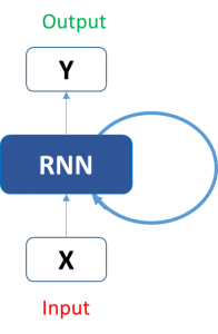
This may seem intimidating at first. But once we unfold it, things start looking a lot simpler:

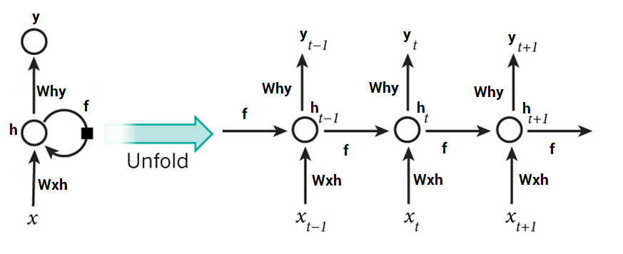It is now easier for us to visualize how these networks are considering the trend of stock prices. This helps us in predicting the prices for the day. Here, every prediction at time t (h_t) is dependent on all previous predictions and the information learned from them. Fairly straightforward, right?

RNNs can solve our purpose of sequence handling to a great extent but not entirely.

Text is another good example of sequence data. Being able to predict what word or phrase comes after a given text could be a very useful asset. We want our models to write Shakespearean sonnets!

Now, RNNs are great when it comes to context that is short or small in nature. But in order to be able to build a story and remember it, our models should be able to understand the context behind the sequences, just like a human brain.

Sequence Prediction using RNN

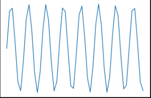
In this article, we will work on a sequence prediction problem using RNN. One of the simplest tasks for this is sine wave prediction. The sequence contains a visible trend and is easy to solve using heuristics. This is what a sine wave looks like:

We will first devise a recurrent neural network from scratch to solve this problem. Our RNN model should also be able to generalize well so we can apply it on other sequence problems.

We will formulate our problem like this – given a sequence of 50 numbers belonging to a sine wave, predict the 51st number in the series. Time to fire up your Jupyter notebook (or your IDE of choice)!

Coding RNN using Python

Step 0: Data Preparation

Ah, the inevitable first step in any data science project – preparing the data before we do anything else.

What does our network model expect the data to be like? It would accept a single sequence of length 50 as input. So the shape of the input data will be:

(number_of_records x length_of_sequence x types_of_sequences)

Here, types_of_sequences is 1, because we have only one type of sequence – the sine wave.

On the other hand, the output would have only one value for each record. This will of course be the 51st value in the input sequence. So it’s shape would be:

(number_of_records x types_of_sequences) #where types_of_sequences is 1

Let’s dive into the code. First, import the necessary libraries:

%pylab inline

import math

To create a sine wave like data, we will use the sine function from Python’s math library:

sin_wave = np.array([math.sin(x) for x in np.arange(200)])

Visualizing the sine wave we’ve just generated:

plt.plot(sin_wave[:50])

X = []
Y = []

seq_len = 50
num_records = len(sin_wave) - seq_len

for i in range(num_records - 50):
    X.append(sin_wave[i:i+seq_len])
    Y.append(sin_wave[i+seq_len])
    
X = np.array(X)
X = np.expand_dims(X, axis=2)

Y = np.array(Y)
Y = np.expand_dims(Y, axis=1)

X.shape, Y.shape

((100, 50, 1), (100, 1))

X_val = []
Y_val = []

for i in range(num_records - 50, num_records):
    X_val.append(sin_wave[i:i+seq_len])
    Y_val.append(sin_wave[i+seq_len])
    
X_val = np.array(X_val)
X_val = np.expand_dims(X_val, axis=2)

Y_val = np.array(Y_val)
Y_val = np.expand_dims(Y_val, axis=1)

learning_rate = 0.0001    
nepoch = 25               
T = 50                   # length of sequence
hidden_dim = 100         
output_dim = 1

bptt_truncate = 5
min_clip_value = -10
max_clip_value = 10

U = np.random.uniform(0, 1, (hidden_dim, T))
W = np.random.uniform(0, 1, (hidden_dim, hidden_dim))
V = np.random.uniform(0, 1, (output_dim, hidden_dim))

def sigmoid(x):
    return 1 / (1 + np.exp(-x))

Step 2: Train the Model

Now that we have defined our model, we can finally move on with training it on our sequence data. We can subdivide the training process into smaller steps, namely:

Step 2.1 : Check the loss on training data
Step 2.1.1 : Forward Pass
Step 2.1.2 : Calculate Error
Step 2.2 : Check the loss on validation data
Step 2.2.1 : Forward Pass
Step 2.2.2 : Calculate Error
Step 2.3 : Start actual training
Step 2.3.1 : Forward Pass
Step 2.3.2 : Backpropagate Error
Step 2.3.3 : Update weights

We need to repeat these steps until convergence. If the model starts to overfit, stop! Or simply pre-define the number of epochs.

Step 2.1: Check the loss on training data

We will do a forward pass through our RNN model and calculate the squared error for the predictions for all records in order to get the loss value.

for epoch in range(nepoch):
    # check loss on train
    loss = 0.0
    
    # do a forward pass to get prediction
    for i in range(Y.shape[0]):
        x, y = X[i], Y[i]                    # get input, output values of each record
        prev_s = np.zeros((hidden_dim, 1))   # here, prev-s is the value of the previous activation of hidden layer; which is initialized as all zeroes
        for t in range(T):
            new_input = np.zeros(x.shape)    # we then do a forward pass for every timestep in the sequence
            new_input[t] = x[t]              # for this, we define a single input for that timestep
            mulu = np.dot(U, new_input)
            mulw = np.dot(W, prev_s)
            add = mulw + mulu
            s = sigmoid(add)
            mulv = np.dot(V, s)
            prev_s = s

    # calculate error 
        loss_per_record = (y - mulv)**2 / 2
        loss += loss_per_record
    loss = loss / float(y.shape[0])

Step 2.2: Check the loss on validation data

We will do the same thing for calculating the loss on validation data (in the same loop):

    # check loss on val
    val_loss = 0.0
    for i in range(Y_val.shape[0]):
        x, y = X_val[i], Y_val[i]
        prev_s = np.zeros((hidden_dim, 1))
        for t in range(T):
            new_input = np.zeros(x.shape)
            new_input[t] = x[t]
            mulu = np.dot(U, new_input)
            mulw = np.dot(W, prev_s)
            add = mulw + mulu
            s = sigmoid(add)
            mulv = np.dot(V, s)
            prev_s = s

        loss_per_record = (y - mulv)**2 / 2
        val_loss += loss_per_record
    val_loss = val_loss / float(y.shape[0])

    print('Epoch: ', epoch + 1, ', Loss: ', loss, ', Val Loss: ', val_loss)

You should get the below output:

Epoch:  1 , Loss:  [[101185.61756671]] , Val Loss:  [[50591.0340148]]
...
...

Step 2.3: Start actual training

We will now start with the actual training of the network. In this, we will first do a forward pass to calculate the errors and a backward pass to calculate the gradients and update them. Let me show you these step-by-step so you can visualize how it works in your mind.

Step 2.3.1: Forward Pass

In the forward pass:

• We first multiply the input with the weights between input and hidden layers
• Add this with the multiplication of weights in the RNN layer. This is because we want to capture the knowledge of the previous timestep
• Pass it through a sigmoid activation function
• Multiply this with the weights between hidden and output layers
• At the output layer, we have a linear activation of the values so we do not explicitly pass the value through an activation layer
• Save the state at the current layer and also the state at the previous timestep in a dictionary

Here is the code for doing a forward pass (note that it is in continuation of the above loop):

    # train model
    for i in range(Y.shape[0]):
        x, y = X[i], Y[i]
    
        layers = []
        prev_s = np.zeros((hidden_dim, 1))
        dU = np.zeros(U.shape)
        dV = np.zeros(V.shape)
        dW = np.zeros(W.shape)
        
        dU_t = np.zeros(U.shape)
        dV_t = np.zeros(V.shape)
        dW_t = np.zeros(W.shape)
        
        dU_i = np.zeros(U.shape)
        dW_i = np.zeros(W.shape)
        
        # forward pass
        for t in range(T):
            new_input = np.zeros(x.shape)
            new_input[t] = x[t]
            mulu = np.dot(U, new_input)
            mulw = np.dot(W, prev_s)
            add = mulw + mulu
            s = sigmoid(add)
            mulv = np.dot(V, s)
            layers.append({'s':s, 'prev_s':prev_s})
            prev_s = s

Step 2.3.2 : Backpropagate Error

After the forward propagation step, we calculate the gradients at each layer, and backpropagate the errors. We will use truncated back propagation through time (TBPTT), instead of vanilla backprop. It may sound complex but its actually pretty straight forward.

The core difference in BPTT versus backprop is that the backpropagation step is done for all the time steps in the RNN layer. So if our sequence length is 50, we will backpropagate for all the timesteps previous to the current timestep.

If you have guessed correctly, BPTT seems very computationally expensive. So instead of backpropagating through all previous timestep , we backpropagate till x timesteps to save computational power. Consider this ideologically similar to stochastic gradient descent, where we include a batch of data points instead of all the data points.

Here is the code for backpropagating the errors:

        # derivative of pred
        dmulv = (mulv - y)
        
        # backward pass
        for t in range(T):
            dV_t = np.dot(dmulv, np.transpose(layers[t]['s']))
            dsv = np.dot(np.transpose(V), dmulv)
            
            ds = dsv
            dadd = add * (1 - add) * ds
            
            dmulw = dadd * np.ones_like(mulw)

            dprev_s = np.dot(np.transpose(W), dmulw)


            for i in range(t-1, max(-1, t-bptt_truncate-1), -1):
                ds = dsv + dprev_s
                dadd = add * (1 - add) * ds

                dmulw = dadd * np.ones_like(mulw)
                dmulu = dadd * np.ones_like(mulu)

                dW_i = np.dot(W, layers[t]['prev_s'])
                dprev_s = np.dot(np.transpose(W), dmulw)

                new_input = np.zeros(x.shape)
                new_input[t] = x[t]
                dU_i = np.dot(U, new_input)
                dx = np.dot(np.transpose(U), dmulu)

                dU_t += dU_i
                dW_t += dW_i
                
            dV += dV_t
            dU += dU_t
            dW += dW_t

Step 2.3.3 : Update weights

Lastly, we update the weights with the gradients of weights calculated. One thing we have to keep in mind that the gradients tend to explode if you don’t keep them in check.This is a fundamental issue in training neural networks, called the exploding gradient problem. So we have to clamp them in a range so that they dont explode. We can do it like this

            if dU.max() > max_clip_value:
                dU[dU > max_clip_value] = max_clip_value
            if dV.max() > max_clip_value:
                dV[dV > max_clip_value] = max_clip_value
            if dW.max() > max_clip_value:
                dW[dW > max_clip_value] = max_clip_value
                
            
            if dU.min() < min_clip_value:
                dU[dU < min_clip_value] = min_clip_value
            if dV.min() < min_clip_value:
                dV[dV < min_clip_value] = min_clip_value
            if dW.min() < min_clip_value:
                dW[dW < min_clip_value] = min_clip_value
        
        # update
        U -= learning_rate * dU
        V -= learning_rate * dV
        W -= learning_rate * dW

On training the above model, we get this output:

Epoch:  1 , Loss:  [[101185.61756671]] , Val Loss:  [[50591.0340148]]
Epoch:  2 , Loss:  [[61205.46869629]] , Val Loss:  [[30601.34535365]]
Epoch:  3 , Loss:  [[31225.3198258]] , Val Loss:  [[15611.65669247]]
Epoch:  4 , Loss:  [[11245.17049551]] , Val Loss:  [[5621.96780111]]
Epoch:  5 , Loss:  [[1264.5157739]] , Val Loss:  [[632.02563908]]
Epoch:  6 , Loss:  [[20.15654115]] , Val Loss:  [[10.05477285]]
Epoch:  7 , Loss:  [[17.13622839]] , Val Loss:  [[8.55190426]]
Epoch:  8 , Loss:  [[17.38870495]] , Val Loss:  [[8.68196484]]
Epoch:  9 , Loss:  [[17.181681]] , Val Loss:  [[8.57837827]]
Epoch:  10 , Loss:  [[17.31275313]] , Val Loss:  [[8.64199652]]
Epoch:  11 , Loss:  [[17.12960034]] , Val Loss:  [[8.54768294]]
Epoch:  12 , Loss:  [[17.09020065]] , Val Loss:  [[8.52993502]]
Epoch:  13 , Loss:  [[17.17370113]] , Val Loss:  [[8.57517454]]
Epoch:  14 , Loss:  [[17.04906914]] , Val Loss:  [[8.50658127]]
Epoch:  15 , Loss:  [[16.96420184]] , Val Loss:  [[8.46794248]]
Epoch:  16 , Loss:  [[17.017519]] , Val Loss:  [[8.49241316]]
Epoch:  17 , Loss:  [[16.94199493]] , Val Loss:  [[8.45748739]]
Epoch:  18 , Loss:  [[16.99796892]] , Val Loss:  [[8.48242177]]
Epoch:  19 , Loss:  [[17.24817035]] , Val Loss:  [[8.6126231]]
Epoch:  20 , Loss:  [[17.00844599]] , Val Loss:  [[8.48682234]]
Epoch:  21 , Loss:  [[17.03943262]] , Val Loss:  [[8.50437328]]
Epoch:  22 , Loss:  [[17.01417255]] , Val Loss:  [[8.49409597]]
Epoch:  23 , Loss:  [[17.20918888]] , Val Loss:  [[8.5854792]]
Epoch:  24 , Loss:  [[16.92068017]] , Val Loss:  [[8.44794633]]
Epoch:  25 , Loss:  [[16.76856238]] , Val Loss:  [[8.37295808]]

Looking good! Time to get the predictions and plot them to get a visual sense of what we’ve designed.

Step 3: Get predictions

We will do a forward pass through the trained weights to get our predictions:

preds = []
for i in range(Y.shape[0]):
    x, y = X[i], Y[i]
    prev_s = np.zeros((hidden_dim, 1))
    # Forward pass
    for t in range(T):
        mulu = np.dot(U, x)
        mulw = np.dot(W, prev_s)
        add = mulw + mulu
        s = sigmoid(add)
        mulv = np.dot(V, s)
        prev_s = s

    preds.append(mulv)
    
preds = np.array(preds)

Plotting these predictions alongside the actual values:

plt.plot(preds[:, 0, 0], 'g')
plt.plot(Y[:, 0], 'r')
plt.show()

This was on the training data. How do we know if our model didn’t overfit? This is where the validation set, which we created earlier, comes into play:

preds = []
for i in range(Y_val.shape[0]):
    x, y = X_val[i], Y_val[i]
    prev_s = np.zeros((hidden_dim, 1))
    # For each time step...
    for t in range(T):
        mulu = np.dot(U, x)
        mulw = np.dot(W, prev_s)
        add = mulw + mulu
        s = sigmoid(add)
        mulv = np.dot(V, s)
        prev_s = s

    preds.append(mulv)
    
preds = np.array(preds)

plt.plot(preds[:, 0, 0], 'g')
plt.plot(Y_val[:, 0], 'r')
plt.show()

Not bad. The predictions are looking impressive. The RMSE score on the validation data is respectable as well:

from sklearn.metrics import mean_squared_error

math.sqrt(mean_squared_error(Y_val[:, 0] * max_val, preds[:, 0, 0] * max_val))

0.127191931509431