Introduction

Predicting how the stock market will perform is one of the most difficult things to do. There are so many factors involved in the prediction – physical factors vs. physhological, rational and irrational behaviour, etc. All these aspects combine to make share prices volatile and very difficult to predict with a high degree of accuracy.

Can we use machine learning as a game changer in this domain? Using features like the latest announcements about an organization, their quarterly revenue results, etc., machine learning techniques have the potential to unearth patterns and insights we didn’t see before, and these can be used to make unerringly accurate predictions.

In this article, we will work with historical data about the stock prices of a publicly listed company. We will implement a mix of machine learning algorithms to predict the future stock price of this company, starting with simple algorithms like averaging and linear regression, and then move on to advanced techniques like Auto ARIMA and LSTM.

The core idea behind this article is to showcase how these algorithms are implemented. I will briefly describe the technique and provide relevant links to brush up on the concepts as and when necessary. In case you’re a newcomer to the world of time series, I suggest going through the following articles first:

• A comprehensive beginner’s guide to create a Time Series Forecast
• A Complete Tutorial on Time Series Modeling
• Free Course: Time Series Forecasting using Python

 

Project to Practice Time Series Forecasting Problem Statement Time Series forecasting & modeling plays an important role in data analysis. Time series analysis is a specialized branch of statistics used extensively in fields such as Econometrics & Operation Research. Time Series is being widely used in analytics & data science. This is specifically designed time series problem for you and the challenge is to forecast traffic. Practice Now

 

Table of Contents

1. 1. Understanding the Problem Statement
   2. Moving Average
   3. Linear Regression
   4. k-Nearest Neighbors
   5. Auto ARIMA
   6. Prophet
   7. Long Short Term Memory (LSTM)

 

Understanding the Problem Statement

We’ll dive into the implementation part of this article soon, but first it’s important to establish what we’re aiming to solve. Broadly, stock market analysis is divided into two parts – Fundamental Analysis and Technical Analysis.

• Fundamental Analysis involves analyzing the company’s future profitability on the basis of its current business environment and financial performance.
• Technical Analysis, on the other hand, includes reading the charts and using statistical figures to identify the trends in the stock market.

As you might have guessed, our focus will be on the technical analysis part. We’ll be using a dataset from Quandl (you can find historical data for various stocks here) and for this particular project, I have used the data for ‘Tata Global Beverages’. Time to dive in!

Note: Here is the dataset I used for the code: Download

We will first load the dataset and define the target variable for the problem:

#import packages
import pandas as pd
import numpy as np

#to plot within notebook
import matplotlib.pyplot as plt
%matplotlib inline

#setting figure size
from matplotlib.pylab import rcParams
rcParams['figure.figsize'] = 20,10

#for normalizing data
from sklearn.preprocessing import MinMaxScaler
scaler = MinMaxScaler(feature_range=(0, 1))

#read the file
df = pd.read_csv('NSE-TATAGLOBAL(1).csv')

#print the head
df.head()

There are multiple variables in the dataset – date, open, high, low, last, close, total_trade_quantity, and turnover.

• The columns Open and Close represent the starting and final price at which the stock is traded on a particular day.
• High, Low and Last represent the maximum, minimum, and last price of the share for the day.
• Total Trade Quantity is the number of shares bought or sold in the day and Turnover (Lacs) is the turnover of the particular company on a given date.

Another important thing to note is that the market is closed on weekends and public holidays.Notice the above table again, some date values are missing – 2/10/2018, 6/10/2018, 7/10/2018. Of these dates, 2nd is a national holiday while 6th and 7th fall on a weekend.

The profit or loss calculation is usually determined by the closing price of a stock for the day, hence we will consider the closing price as the target variable. Let’s plot the target variable to understand how it’s shaping up in our data:

#setting index as date
df['Date'] = pd.to_datetime(df.Date,format='%Y-%m-%d')
df.index = df['Date']

#plot
plt.figure(figsize=(16,8))
plt.plot(df['Close'], label='Close Price history')

In the upcoming sections, we will explore these variables and use different techniques to predict the daily closing price of the stock.

 

Moving Average

Introduction

‘Average’ is easily one of the most common things we use in our day-to-day lives. For instance, calculating the average marks to determine overall performance, or finding the average temperature of the past few days to get an idea about today’s temperature – these all are routine tasks we do on a regular basis. So this is a good starting point to use on our dataset for making predictions.

The predicted closing price for each day will be the average of a set of previously observed values. Instead of using the simple average, we will be using the moving average technique which uses the latest set of values for each prediction. In other words, for each subsequent step, the predicted values are taken into consideration while removing the oldest observed value from the set. Here is a simple figure that will help you understand this with more clarity.

We will implement this technique on our dataset. The first step is to create a dataframe that contains only the Date and Close price columns, then split it into train and validation sets to verify our predictions.

 

Implementation

 

Just checking the RMSE does not help us in understanding how the model performed. Let’s visualize this to get a more intuitive understanding. So here is a plot of the predicted values along with the actual values.

#plot
valid['Predictions'] = 0
valid['Predictions'] = preds
plt.plot(train['Close'])
plt.plot(valid[['Close', 'Predictions']])

 

Inference

The RMSE value is close to 105 but the results are not very promising (as you can gather from the plot). The predicted values are of the same range as the observed values in the train set (there is an increasing trend initially and then a slow decrease).

In the next section, we will look at two commonly used machine learning techniques – Linear Regression and kNN, and see how they perform on our stock market data.

 

Linear Regression

Introduction

The most basic machine learning algorithm that can be implemented on this data is linear regression. The linear regression model returns an equation that determines the relationship between the independent variables and the dependent variable.

The equation for linear regression can be written as:

Here, x₁, x₂,….x_n represent the independent variables while the coefficients θ₁, θ₂, …. θ_n  represent the weights. You can refer to the following article to study linear regression in more detail:

• A comprehensive beginners guide for Linear, Ridge and Lasso Regression.

For our problem statement, we do not have a set of independent variables. We have only the dates instead. Let us use the date column to extract features like – day, month, year,  mon/fri etc. and then fit a linear regression model.

Implementation

We will first sort the dataset in ascending order and then create a separate dataset so that any new feature created does not affect the original data.

#setting index as date values
df['Date'] = pd.to_datetime(df.Date,format='%Y-%m-%d')
df.index = df['Date']

#sorting
data = df.sort_index(ascending=True, axis=0)

#creating a separate dataset
new_data = pd.DataFrame(index=range(0,len(df)),columns=['Date', 'Close'])

for i in range(0,len(data)):
    new_data['Date'][i] = data['Date'][i]
    new_data['Close'][i] = data['Close'][i]

 

#create features
from fastai.structured import  add_datepart
add_datepart(new_data, 'Date')
new_data.drop('Elapsed', axis=1, inplace=True)  #elapsed will be the time stamp

This creates features such as:

‘Year’, ‘Month’, ‘Week’, ‘Day’, ‘Dayofweek’, ‘Dayofyear’, ‘Is_month_end’, ‘Is_month_start’, ‘Is_quarter_end’, ‘Is_quarter_start’,  ‘Is_year_end’, and  ‘Is_year_start’.

Note: I have used add_datepart from fastai library. If you do not have it installed, you can simply use the command pip install fastai. Otherwise, you can create these feature using simple for loops in python. I have shown an example below.

Apart from this, we can add our own set of features that we believe would be relevant for the predictions. For instance, my hypothesis is that the first and last days of the week could potentially affect the closing price of the stock far more than the other days. So I have created a feature that identifies whether a given day is Monday/Friday or Tuesday/Wednesday/Thursday. This can be done using the following lines of code:

new_data['mon_fri'] = 0
for i in range(0,len(new_data)):
    if (new_data['Dayofweek'][i] == 0 or new_data['Dayofweek'][i] == 4):
        new_data['mon_fri'][i] = 1
    else:
        new_data['mon_fri'][i] = 0

If the day of week is equal to 0 or 4, the column value will be 1, otherwise 0. Similarly, you can create multiple features. If you have some ideas for features that can be helpful in predicting stock price, please share in the comment section.

We will now split the data into train and validation sets to check the performance of the model.

#split into train and validation
train = new_data[:987]
valid = new_data[987:]

x_train = train.drop('Close', axis=1)
y_train = train['Close']
x_valid = valid.drop('Close', axis=1)
y_valid = valid['Close']

#implement linear regression
from sklearn.linear_model import LinearRegression
model = LinearRegression()
model.fit(x_train,y_train)

Results

#make predictions and find the rmse
preds = model.predict(x_valid)
rms=np.sqrt(np.mean(np.power((np.array(y_valid)-np.array(preds)),2)))
rms

121.16291596523156

The RMSE value is higher than the previous technique, which clearly shows that linear regression has performed poorly. Let’s look at the plot and understand why linear regression has not done well:

#plot
valid['Predictions'] = 0
valid['Predictions'] = preds

valid.index = new_data[987:].index
train.index = new_data[:987].index

plt.plot(train['Close'])
plt.plot(valid[['Close', 'Predictions']])

Inference

Linear regression is a simple technique and quite easy to interpret, but there are a few obvious disadvantages. One problem in using regression algorithms is that the model overfits to the date and month column. Instead of taking into account the previous values from the point of prediction, the model will consider the value from the same date a month ago, or the same date/month a year ago.

As seen from the plot above, for January 2016 and January 2017, there was a drop in the stock price. The model has predicted the same for January 2018. A linear regression technique can perform well for problems such as Big Mart sales where the independent features are useful for determining the target value.

 

k-Nearest Neighbours

Introduction

Another interesting ML algorithm that one can use here is kNN (k nearest neighbours). Based on the independent variables, kNN finds the similarity between new data points and old data points. Let me explain this with a simple example.

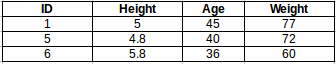
Consider the height and age for 11 people. On the basis of given features (‘Age’ and ‘Height’), the table can be represented in a graphical format as shown below:

To determine the weight for ID #11, kNN considers the weight of the nearest neighbors of this ID. The weight of ID #11 is predicted to be the average of it’s neighbors. If we consider three neighbours (k=3) for now, the weight for ID#11 would be = (77+72+60)/3 = 69.66 kg.

 

For a detailed understanding of kNN, you can refer to the following articles:

• Introduction to k-Nearest Neighbors: Simplified 

• A Practical Introduction to K-Nearest Neighbors Algorithm for Regression

 

Implementation

#importing libraries
from sklearn import neighbors
from sklearn.model_selection import GridSearchCV
from sklearn.preprocessing import MinMaxScaler
scaler = MinMaxScaler(feature_range=(0, 1))

Using the same train and validation set from the last section:

#scaling data
x_train_scaled = scaler.fit_transform(x_train)
x_train = pd.DataFrame(x_train_scaled)
x_valid_scaled = scaler.fit_transform(x_valid)
x_valid = pd.DataFrame(x_valid_scaled)

#using gridsearch to find the best parameter
params = {'n_neighbors':[2,3,4,5,6,7,8,9]}
knn = neighbors.KNeighborsRegressor()
model = GridSearchCV(knn, params, cv=5)

#fit the model and make predictions
model.fit(x_train,y_train)
preds = model.predict(x_valid)

Results

#rmse
rms=np.sqrt(np.mean(np.power((np.array(y_valid)-np.array(preds)),2)))
rms

115.17086550026721

There is not a huge difference in the RMSE value, but a plot for the predicted and actual values should provide a more clear understanding.

#plot
valid['Predictions'] = 0
valid['Predictions'] = preds
plt.plot(valid[['Close', 'Predictions']])
plt.plot(train['Close'])

Inference

The RMSE value is almost similar to the linear regression model and the plot shows the same pattern. Like linear regression, kNN also identified a drop in January 2018 since that has been the pattern for the past years. We can safely say that regression algorithms have not performed well on this dataset.

Let’s go ahead and look at some time series forecasting techniques to find out how they perform when faced with this stock prices prediction challenge.

 

Auto ARIMA

Introduction

ARIMA is a very popular statistical method for time series forecasting. ARIMA models take into account the past values to predict the future values. There are three important parameters in ARIMA:

• p (past values used for forecasting the next value)
• q (past forecast errors used to predict the future values)
• d (order of differencing)

Parameter tuning for ARIMA consumes a lot of time. So we will use auto ARIMA which automatically selects the best combination of (p,q,d) that provides the least error. To read more about how auto ARIMA works, refer to this article:

• Build High Performance Time Series Models using Auto ARIMA

 

Implementation

from pyramid.arima import auto_arima

data = df.sort_index(ascending=True, axis=0)

train = data[:987]
valid = data[987:]

training = train['Close']
validation = valid['Close']

model = auto_arima(training, start_p=1, start_q=1,max_p=3, max_q=3, m=12,start_P=0, seasonal=True,d=1, D=1, trace=True,error_action='ignore',suppress_warnings=True)
model.fit(training)

forecast = model.predict(n_periods=248)
forecast = pd.DataFrame(forecast,index = valid.index,columns=['Prediction'])

 

Results

rms=np.sqrt(np.mean(np.power((np.array(valid['Close'])-np.array(forecast['Prediction'])),2)))
rms

44.954584993246954

 

#plot
plt.plot(train['Close'])
plt.plot(valid['Close'])
plt.plot(forecast['Prediction'])

Inference

As we saw earlier, an auto ARIMA model uses past data to understand the pattern in the time series. Using these values, the model captured an increasing trend in the series. Although the predictions using this technique are far better than that of the previously implemented machine learning models, these predictions are still not close to the real values.

As its evident from the plot, the model has captured a trend in the series, but does not focus on the seasonal part. In the next section, we will implement a time series model that takes both trend and seasonality of a series into account.

 

Prophet

Introduction

There are a number of time series techniques that can be implemented on the stock prediction dataset, but most of these techniques require a lot of data preprocessing before fitting the model. Prophet, designed and pioneered by Facebook, is a time series forecasting library that requires no data preprocessing and is extremely simple to implement. The input for Prophet is a dataframe with two columns: date and target (ds and y).

Prophet tries to capture the seasonality in the past data and works well when the dataset is large. Here is an interesting article that explains Prophet in a simple and intuitive manner:

• Generate Quick and Accurate Time Series Forecasts using Facebook’s Prophet.

Implementation

#importing prophet
from fbprophet import Prophet

#creating dataframe
new_data = pd.DataFrame(index=range(0,len(df)),columns=['Date', 'Close'])

for i in range(0,len(data)):
    new_data['Date'][i] = data['Date'][i]
    new_data['Close'][i] = data['Close'][i]

new_data['Date'] = pd.to_datetime(new_data.Date,format='%Y-%m-%d')
new_data.index = new_data['Date']

#preparing data
new_data.rename(columns={'Close': 'y', 'Date': 'ds'}, inplace=True)

#train and validation
train = new_data[:987]
valid = new_data[987:]

#fit the model
model = Prophet()
model.fit(train)

#predictions
close_prices = model.make_future_dataframe(periods=len(valid))
forecast = model.predict(close_prices)

Results

#rmse
forecast_valid = forecast['yhat'][987:]
rms=np.sqrt(np.mean(np.power((np.array(valid['y'])-np.array(forecast_valid)),2)))
rms

57.494461930575149

#plot
valid['Predictions'] = 0
valid['Predictions'] = forecast_valid.values

plt.plot(train['y'])
plt.plot(valid[['y', 'Predictions']])

Inference

Prophet (like most time series forecasting techniques) tries to capture the trend and seasonality from past data. This model usually performs well on time series datasets, but fails to live up to it’s reputation in this case.

As it turns out, stock prices do not have a particular trend or seasonality. It highly depends on what is currently going on in the market and thus the prices rise and fall. Hence forecasting techniques like ARIMA, SARIMA and Prophet would not show good results for this particular problem.

Let us go ahead and try another advanced technique – Long Short Term Memory (LSTM).

 

Long Short Term Memory (LSTM)

Introduction

LSTMs are widely used for sequence prediction problems and have proven to be extremely effective. The reason they work so well is because LSTM is able to store past information that is important, and forget the information that is not. LSTM has three gates:

• The input gate: The input gate adds information to the cell state
• The forget gate: It removes the information that is no longer required by the model
• The output gate: Output Gate at LSTM selects the information to be shown as output
  

For a more detailed understanding of LSTM and its architecture, you can go through the below article:

• Introduction to Long Short Term Memory

For now, let us implement LSTM as a black box and check it’s performance on our particular data.

 

Implementation

#importing required libraries
from sklearn.preprocessing import MinMaxScaler
from keras.models import Sequential
from keras.layers import Dense, Dropout, LSTM

#creating dataframe
data = df.sort_index(ascending=True, axis=0)
new_data = pd.DataFrame(index=range(0,len(df)),columns=['Date', 'Close'])
for i in range(0,len(data)):
    new_data['Date'][i] = data['Date'][i]
    new_data['Close'][i] = data['Close'][i]

#setting index
new_data.index = new_data.Date
new_data.drop('Date', axis=1, inplace=True)

#creating train and test sets
dataset = new_data.values

train = dataset[0:987,:]
valid = dataset[987:,:]

#converting dataset into x_train and y_train
scaler = MinMaxScaler(feature_range=(0, 1))
scaled_data = scaler.fit_transform(dataset)

x_train, y_train = [], []
for i in range(60,len(train)):
    x_train.append(scaled_data[i-60:i,0])
    y_train.append(scaled_data[i,0])
x_train, y_train = np.array(x_train), np.array(y_train)

x_train = np.reshape(x_train, (x_train.shape[0],x_train.shape[1],1))

# create and fit the LSTM network
model = Sequential()
model.add(LSTM(units=50, return_sequences=True, input_shape=(x_train.shape[1],1)))
model.add(LSTM(units=50))
model.add(Dense(1))

model.compile(loss='mean_squared_error', optimizer='adam')
model.fit(x_train, y_train, epochs=1, batch_size=1, verbose=2)

#predicting 246 values, using past 60 from the train data
inputs = new_data[len(new_data) - len(valid) - 60:].values
inputs = inputs.reshape(-1,1)
inputs  = scaler.transform(inputs)

X_test = []
for i in range(60,inputs.shape[0]):
    X_test.append(inputs[i-60:i,0])
X_test = np.array(X_test)

X_test = np.reshape(X_test, (X_test.shape[0],X_test.shape[1],1))
closing_price = model.predict(X_test)
closing_price = scaler.inverse_transform(closing_price)

Results

rms=np.sqrt(np.mean(np.power((valid-closing_price),2)))
rms

11.772259608962642

#for plotting
train = new_data[:987]
valid = new_data[987:]
valid['Predictions'] = closing_price
plt.plot(train['Close'])
plt.plot(valid[['Close','Predictions']])

 

Inference

Wow! The LSTM model can be tuned for various parameters such as changing the number of LSTM layers, adding dropout value or increasing the number of epochs. But are the predictions from LSTM enough to identify whether the stock price will increase or decrease? Certainly not!

As I mentioned at the start of the article, stock price is affected by the news about the company and other factors like demonetization or merger/demerger of the companies. There are certain intangible factors as well which can often be impossible to predict beforehand.

 

End Notes

Time series forecasting is a very intriguing field to work with, as I have realized during my time writing these articles. There is a perception in the community that it’s a complex field, and while there is a grain of truth in there, it’s not so difficult once you get the hang of the basic techniques.

I am interested in finding out how LSTM works on a different kind of time series problem and encourage you to try it out on your own as well. If you have any questions, feel free to connect with me in the comments section below.