Introduction

Buying a new product or testing a new technique but not sure how it stacks up against the alternatives? It’s an all too familiar situation for most of us. Most of the options sound similar to each other so picking the best out of the lot is a challenge.

Consider a scenario where we have three medical treatments to apply on patients with similar diseases. Once we have the test results, one approach is to assume that the treatment which took the least time to cure the patients is the best among them. What if some of these patients had already been partially cured, or if any other medication was already working on them?

In order to make a confident and reliable decision, we will need evidence to support our approach. This is where the concept of ANOVA comes into play.

Source: Megapixl

In this article, I’ll introduce you to the different ANOVA techniques used for making the best decisions. We’ll take a few cases and try to understand the techniques for getting the results. We will also be leveraging the use of Excel to understand these concepts. You must know the basics of statistics to understand this topic. Knowledge of t-tests and Hypothesis testing would be an additional benefit.

And we believe the best way to learn statistics is by doing. That’s the way we follow in the ‘Introduction to Data Science‘ course where we provide a comprehensive introduction to statistics – both descriptive and inferential.

So, let’s begin!

 

Table of Contents

1. Introduction to ANOVA
2. Terminologies related to ANOVA you need to know
   • Grand Mean
   • Hypothesis
   • Between Group variability
   • Within Group variability
   • F-Statistic
3. One-way ANOVA
   • Limitations of One-way ANOVA
   • Steps to perform One-way ANOVA in Excel
4. Two-way ANOVA
   • Steps to perform Two-way ANOVA in Excel
5. MANOVA
   • Steps to perform MANOVA in Excel

Introduction to ANOVA

A common approach to figure out a reliable treatment method would be to analyse the days it took the patients to be cured. We can use a statistical technique which can compare these three treatment samples and depict how different these samples are from one another. Such a technique, which compares the samples on the basis of their means, is called ANOVA.

Analysis of variance (ANOVA) is a statistical technique that is used to check if the means of two or more groups are significantly different from each other. ANOVA checks the impact of one or more factors by comparing the means of different samples.

We can use ANOVA to prove/disprove if all the medication treatments were equally effective or not.

Source: Questionpro

Another measure to compare the samples is called a t-test. When we have only two samples, t-test and ANOVA give the same results. However, using a t-test would not be reliable in cases where there are more than 2 samples. If we conduct multiple t-tests for comparing more than two samples, it will have a compounded effect on the error rate of the result.

 

Terminologies related to ANOVA you need to know

Before we get started with the applications of ANOVA, I would like to introduce some common terminologies used in the technique.

Grand Mean

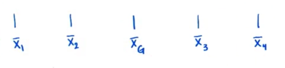
Mean is a simple or arithmetic average of a range of values. There are two kinds of means that we use in ANOVA calculations, which are separate sample means  and the grand mean  . The grand mean is the mean of sample means or the mean of all observations combined, irrespective of the sample.

 

Hypothesis

Considering our above medication example, we can assume that there are 2 possible cases – either the medication will have an effect on the patients or it won’t. These statements are called Hypothesis. A hypothesis is an educated guess about something in the world around us. It should be testable either by experiment or observation.

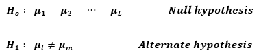
Just like any other kind of hypothesis that you might have studied in statistics, ANOVA also uses a Null hypothesis and an Alternate hypothesis. The Null hypothesis in ANOVA is valid when all the sample means are equal, or they don’t have any significant difference. Thus, they can be considered as a part of a larger set of the population. On the other hand, the alternate hypothesis is valid when at least one of the sample means is different from the rest of the sample means. In mathematical form, they can be represented as:

 

where  belong to any two sample means out of all the samples considered for the test. In other words, the null hypothesis states that all the sample means are equal or the factor did not have any significant effect on the results. Whereas, the alternate hypothesis states that at least one of the sample means is different from another. But we still can’t tell which one specifically. For that, we will use other methods that we will discuss later in this article.

 

Between Group Variability

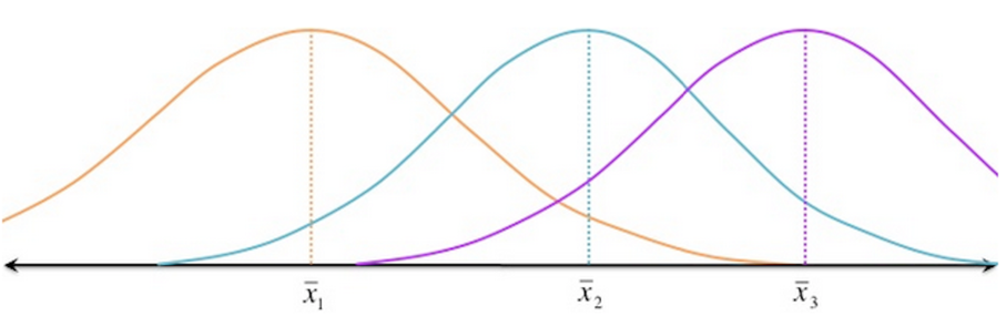
Consider the distributions of the below two samples. As these samples overlap, their individual means won’t differ by a great margin. Hence the difference between their individual means and grand mean won’t be significant enough.

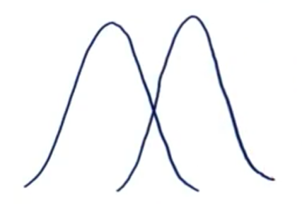
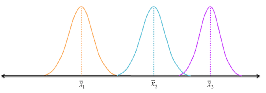
Now consider these two sample distributions. As the samples differ from each other by a big margin, their individual means would also differ. The difference between the individual means and grand mean would therefore also be significant.

 

Such variability between the distributions called Between-group variability. It refers to variations between the distributions of individual groups (or levels) as the values within each group are different.

Each sample is looked at and the difference between its mean and grand mean is calculated to calculate the variability. If the distributions overlap or are close, the grand mean will be similar to the individual means whereas if the distributions are far apart, difference between means and grand mean would be large.

Source: Psychstat – Missouri State

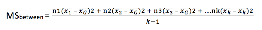
We will calculate Between Group Variability just as we calculate the standard deviation. Given the sample means and Grand mean, we can calculate it as:

Source: Udacity

We also want to weigh each squared deviation by the size of the sample. In other words, a deviation is given greater weight if it’s from a larger sample. Hence, we’ll multiply each squared deviation by each sample size and add them up. This is called the sum-of-squares for between-group variability 

 

There’s one more thing we have to do to derive a good measure of between-group variability. Again, recall how we calculate the sample standard deviation.

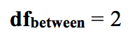
We find the sum of each squared deviation and divide it by the degrees of freedom. For our between-group variability, we will find each squared deviation, weigh them by their sample size, sum them up, and divide by the degrees of freedom (), which in the case of between-group variability is the number of sample means (k) minus 1.

 

Within Group Variability

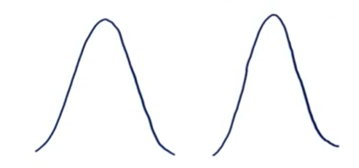
Consider the given distributions of three samples. As the spread (variability) of each sample is increased, their distributions overlap and they become part of a big population.

Now consider another distribution of the same three samples but with less variability. Although the means of samples are similar to the samples in the above image, they seem to belong to different populations.

Source: TurntheWheelsandBox

Such variations within a sample are denoted by Within-group variation. It refers to variations caused by differences within individual groups (or levels) as not all the values within each group are the same. Each sample is looked at on its own and variability between the individual points in the sample is calculated. In other words, no interactions between samples are considered.

We can measure Within-group variability by looking at how much each value in each sample differs from its respective sample mean. So first, we’ll take the squared deviation of each value from its respective sample mean and add them up. This is the sum of squares for within-group variability.

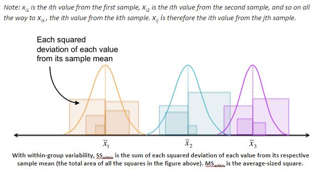
Source: TurntheWheelsandBox

Like between-group variability, we then divide the sum of squared deviations by the degrees of freedom  to find a less-biased estimator for the average squared deviation (essentially, the average-sized square from the figure above). Again, this quotient is called the mean square, but for within-group variability: . This time, the degrees of freedom is the sum of the sample sizes (N) minus the number of samples (k). Another way to look at degrees of freedom is that we have the total number of values (N), and subtract 1 for each sample:

 

F-Statistic

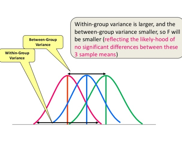
The statistic which measures if the means of different samples are significantly different or not is called the F-Ratio. Lower the F-Ratio, more similar are the sample means. In that case, we cannot reject the null hypothesis.

F = Between group variability / Within group variability

This above formula is pretty intuitive. The numerator term in the F-statistic calculation defines the between-group variability. As we read earlier, as between group variability increases, sample means grow further apart from each other. In other words, the samples are more probable to be belonging to totally different populations.

This F-statistic calculated here is compared with the F-critical value for making a conclusion. In terms of our medication example, if the value of the calculated F-statistic is more than the F-critical value (for a specific α/significance level), then we reject the null hypothesis and can say that the treatment had a significant effect.

Source: Dr. Asim’s Anatomy Cafe

Unlike the z and t-distributions, the F-distribution does not have any negative values because between and within-group variability are always positive due to squaring each deviation.

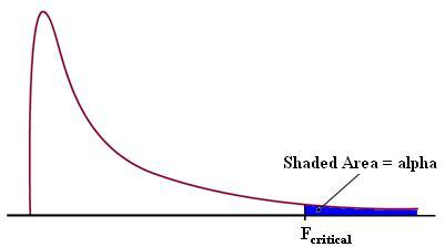
Source: Statistics How To

Therefore, there is only one critical region, in the right tail (shown as the blue shaded region above). If the F-statistic lands in the critical region, we can conclude that the means are significantly different and we reject the null hypothesis. Again, we have to find the critical value to determine the cut-off for the critical region. We’ll use the F-table for this purpose.

We need to look at different F-values for each alpha/significance level because the F-critical value is a function of two things:   and .

One Way ANOVA

As we now understand the basic terminologies behind ANOVA, let’s dive deep into its implementation using a few examples.

A recent study claims that using music in a class enhances the concentration and consequently helps students absorb more information. As a teacher, your first reaction would be skepticism.

What if it affected the results of the students in a negative way? Or what kind of music would be a good choice for this? Considering all this, it would be immensely helpful to have some proof that it actually works.

To figure this out, we decided to implement it on a smaller group of randomly selected students from three different classes. The idea is similar to conducting a survey. We take three different groups of ten randomly selected students (all of the same age) from three different classrooms. Each classroom was provided with a different environment for students to study. Classroom A had constant music being played in the background, classroom B had variable music being played and classroom C was a regular class with no music playing. After one month, we conducted a test for all the three groups and collected their test scores. The test scores that we obtained were as follows:

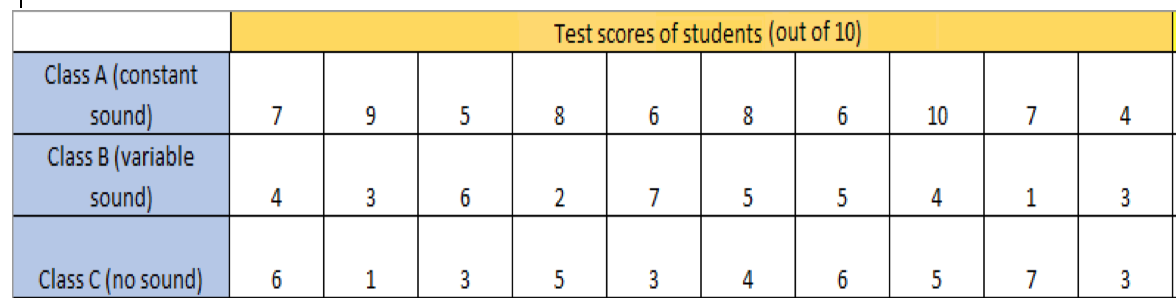
Now, we will calculate the means and the Grand mean.

So, in our case, 

 

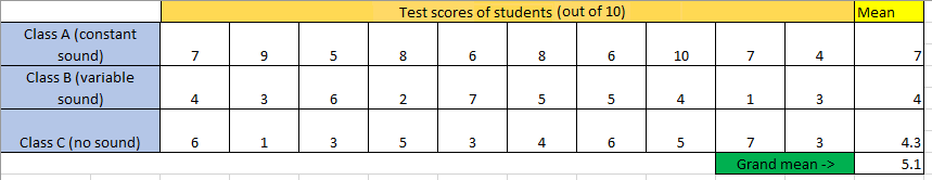
Looking at the above table, we might assume that the mean score of students from Group A is definitely greater than the other two groups, so the treatment must be helpful. Maybe it’s true, but there is also a slight chance that we happened to select the best students from class A, which resulted in better test scores (remember, the selection was done at random). This leads to a few questions, like:

1. How do we decide that these three groups performed differently because of the different situations and not merely by chance?
2. In a statistical sense, how different are these three samples from each other?
3. What is the probability of group A students performing so differently than the other two groups?

To answer all these questions, first we will calculate the F-statistic which can be expressed as the ratio of Between Group variability and Within Group Variability.

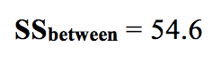
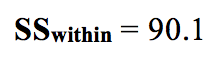
Let’s complete the ANOVA test for our example with  = 0.05.

Limitations of one-way ANOVA

A one-way ANOVA tells us that at least two groups are different from each other. But it won’t tell us which groups are different. If our test returns a significant f-statistic, we may need to run a post-hoc test to tell us exactly which groups have a difference in means. Below I have mentioned the steps to perform one-way ANOVA in Excel along with a post-hoc test.

Steps to perform one-way ANOVA with post-hoc test in Excel 2013

Step 1: Input your data into columns or rows in Excel. For example, if three groups of students for music treatment are being tested, spread the data into three columns.

Step 2: Click the “Data” tab and then click “Data Analysis.” If you don’t see Data Analysis, load the ‘Data Analysis Toolpak’ add-in.

Step 3: Click “ANOVA Single Factor” and then click “OK.”

Step 4: Type an input range into the Input Range box. For example, if the data is in cells A1 to C10, type “A1:C10” into the box. Check the “Labels in first row” if we have column headers, and select the Rows radio button if the data is in rows.

Step 5: Select an output range. For example, click the “New Worksheet” radio button.

Step 6: Choose an alpha level. For most hypothesis tests, 0.05 is standard.

Step 7: Click “OK.” The results from ANOVA will appear in the worksheet.

Results for our example look like this:

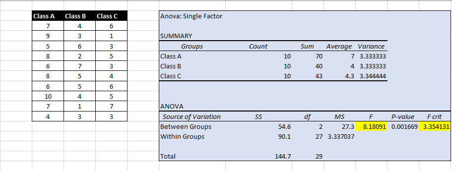
Here, we can see that the F-value is greater than the F-critical value for the alpha level selected (0.05). Therefore, we have evidence to reject the null hypothesis and say that at least one of the three samples have significantly different means and thus belong to an entirely different population.

Another measure for ANOVA is the p-value. If the p-value is less than the alpha level selected (which it is, in our case), we reject the Null Hypothesis.

There are various methods for finding out which are the samples that represent two different populations. I’ll list some for you:

1. Bonferroni approach
2. Least significant difference test
3. Tukey’s HSD

We won’t be covering all of these here in this article but I suggest you go through them.

Now to check which samples had different means we will take the Bonferroni approach and perform the post hoc test in Excel.

Step 8: Again, click on “Data Analysis” in the “Data” tab and select “t-Test: Two-Sample Assuming Equal Variances” and click “OK.”

Step 9: Input the range of Class A column in Variable 1 Range box, and range of Class B column in Variable 2 Range box. Check the “Labels” if you have column headers in the first row.

Step 10: Select an output range. For example, click the “New Worksheet” radio button.

Step 11: Perform the same steps (Step 8 to step 10) for Columns of Class B – Class C and Class A – Class C.

The results will look like this:

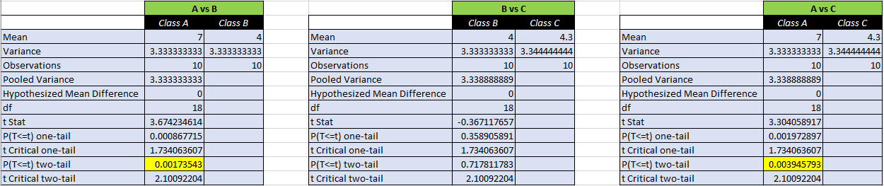
Here, we can see that the p-value of (A vs B) and (A vs C) is less than the alpha level selected (alpha = 0.05). This means that groups A and B & groups A and C have less than 5% chance of belonging to the same population. Whereas for (B vs C) it is much greater than the significance level. This means that B and C belong to the same population. So, it is clear that A (constant music group) belongs to an entirely different population. Or we can say that the constant music had a significant effect on the performance of students.

Voila! The music experiment actually helped in improving the results of the students.

Another effect size measure for one-way ANOVA is called Eta squared. It works in the same way as R2 for t-tests. It is used to calculate how much proportion of the variability between the samples is due to the between group difference. It is calculated as:

For the above example:

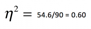
Hence 60% of the difference between the scores is because of the approach that was used. Rest 40% is unknown. Hence Eta square helps us conclude whether the independent variable is really having an impact on the dependent variable or the difference is due to chance or any other factor.

There are commonly two types of ANOVA tests for univariate analysis – One-Way ANOVA and Two-Way ANOVA. One-way ANOVA is used when we are interested in studying the effect of one independent variable (IDV)/factor on a population, whereas Two-way ANOVA is used for studying the effects of two factors on a population at the same time. For multivariate analysis, such a technique is called MANOVA or Multi-variate ANOVA.

 

Two-Way ANOVA:

Using one-way ANOVA, we found out that the music treatment was helpful in improving the test results of our students. But this treatment was conducted on students of the same age. What if the treatment was to affect different age groups of students in different ways? Or maybe the treatment had varying effects depending upon the teacher who taught the class.

Moreover, how can we be sure as to which factor(s) is affecting the results of the students more? Maybe the age group is a more dominant factor responsible for a student’s performance than the music treatment.

For such cases, when the outcome or dependent variable (in our case the test scores) is affected by two independent variables/factors we use a slightly modified technique called two-way ANOVA.

In the one-way ANOVA test, we found out that the group subjected to ‘variable music’ and ‘no music at all’ performed more or less equally. It means that the variable music treatment did not have any significant effect on the students.

So, while performing two-way ANOVA we will not consider the “variable music” treatment for simplicity of calculation. Rather a new factor, age, will be introduced to find out how the treatment performs when applied to students of different age groups. This time our dataset looks like this:

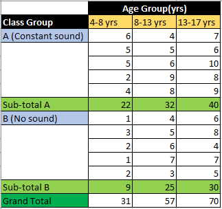
Here, there are two factors – class group and age group with two and three levels respectively. So we now have six different groups of students based on different permutations of class groups and age groups and each different group has a sample size of 5 students.

A few questions that two-way ANOVA can answer about this dataset are:

1. Is music treatment the main factor affecting performance? In other words, do groups subjected to different music differ significantly in their test performance?
2. Is age the main factor affecting performance? In other words, do students of different age differ significantly in their test performance?
3. Is there a significant interaction between the factors? In other words, how do age and music interact with regard to a student’s test performance? For example, it might be that younger students and elder students reacted differently to such a music treatment.
4. Can any differences in one factor be found within another factor? In other words, can any differences in music and test performance be found in different age groups?

Two-way ANOVA tells us about the main effect and the interaction effect. The main effect is similar to a one-way ANOVA where the effect of music and age would be measured separately. Whereas, the interaction effect is the one where both music and age are considered at the same time.

That’s why a two-way ANOVA can have up to three hypotheses, which are as follows:

Two null hypotheses will be tested if we have placed only one observation in each cell. For this example, those hypotheses will be:
H1: All the music treatment groups have equal mean score.
H2: All the age groups have equal mean score.

For multiple observations in cells, we would also be testing a third hypothesis:
H3: The factors are independent or the interaction effect does not exist.

An F-statistic is computed for each hypothesis we are testing.

Before we proceed with the calculation, have a look at the image below. It will help us better understand the terms used in the formulas.

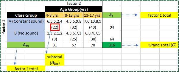
The table shown above is known as a contingency table. Here, represents the total of the samples based only on factor 1, and represents the total of sample based only on factor 2. We will see in some time that these two are responsible for the main effect produced. Also, a term  is introduced which represents the subtotal of factor 1 and factor 2. This term will be responsible for the interaction effect produced when both the factors are considered at the same time. And we are already familiar with the , which is the sum of all the observations (test scores), irrespective of the factors.

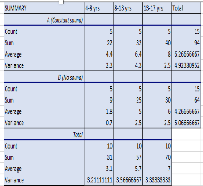
We have calculated all the means – sound class mean, age group mean and mean of every group combination in the above table.

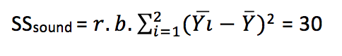
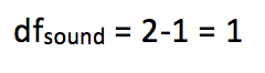
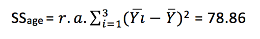
Now, calculate the sum of squares (SS) and degrees of freedom (df) for sound class, age group and interaction between factor and levels.

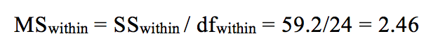
We already know how to calculate SS (within)/df (within) in our one-way ANOVA section, but in two-way ANOVA the formula is different. Let’s look at the calculation of two-way ANOVA:

 

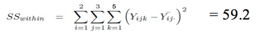
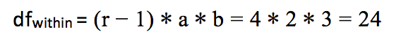
In two-way ANOVA, we also calculate SS_interaction and df_interaction which defines the combined effect of the two factors.

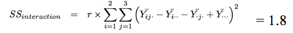
Since we have more than one source of variation (main effects and interaction effects), it is obvious that we will have more than one F-statistic also.

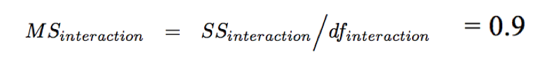
Now using these variances, we compute the value of F-statistic for the main and interaction effect. So, the values of f-statistic are,

F1 = 12.16

F2 = 15.98

F12 = 0.36

We can see the critical values from the table

Fcrit1 = 4.25

Fcrit2 = 3.40

Fcrit12 = 3.40

If, for a particular effect, its F value is greater than its respective F-critical value (calculated using the F-Table), then we reject the null hypothesis for that particular effect.

 

Steps to perform two-way ANOVA in Excel 2013:

Step 1: Click the “Data” tab and then click “Data Analysis.” If you don’t see the Data analysis option, install the Data Analysis Toolpak.

Step 2: Click “ANOVA two factor with replication” and then click “OK.” The two-way ANOVA window will open.

Step 3: Type an Input Range into the Input Range box. For example, if your data is in cells A1 to A25, type “A1:A25” into the Input Range box. Make sure you include all of your data, including headers and group names.

Step 4: Type a number in the “Rows per sample” box. Rows per sample is actually a bit misleading. What this is asking you is how many individuals are in each group. For example, if you have 5 individuals in each age group, you would type “5” into the Rows per Sample box.

Step 5: Select an Output Range. For example, click the “new worksheet” radio button to display the data in a new worksheet.

Step 6: Select an alpha level. In most cases, an alpha level of 0.05 (5 percent) works for most tests.

Step 7: Click “OK” to run the two-way ANOVA. The data will be returned in your specified output range.

Step 8: Read the results. To figure out if you are going to reject the null hypothesis or not, you’ll basically be looking at two factors:

1. If the F-value (F)is larger than the f critical value (F crit)
2. If the p-value is smaller than your chosen alpha level.

And you are done!

Note: We don’t only have to have two variables to run a two-way ANOVA in Excel 2013. We can also use the same function for three, four, five or more number of variables.

The results for two-way ANOVA test on our example look like this:

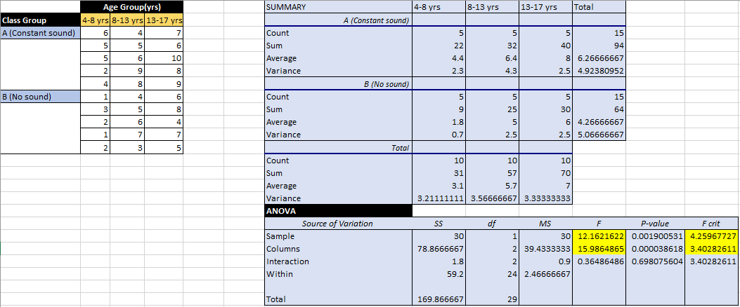
As you can see in the highlighted cells in the image above, the F-value for sample and column, i.e. factor 1 (music) and factor 2 (age) respectively, are higher than their F-critical values. This means that the factors have a significant effect on the results of the students and thus we can reject the null hypothesis for the factors.

Also, the F-value for interaction effect is quite less than its F-critical value, so we can conclude that music and age did not have any combined effect on the population.

 

Multi-variate ANOVA (MANOVA):

Until now, we were making conclusions on the performance of students based on just one test. Could there be a possibility that the music treatment helped improve the results of a subject like mathematics but would affect the results adversely for a theoretical subject like history?

How can we be sure that the treatment won’t be biased in such a case? So again, we take two groups of randomly selected students from a class and subject each group to one kind of music environment, i.e., constant music and no music. But now we thought of conducting two tests (maths and history), instead of just one. This way we can be sure about how the treatment would work for different kind of subjects.

We can say that one IDV/factor (music) will be affecting two dependent variables (maths scores and history scores) now. This kind of a problem comes under a multivariate case and the technique we will use to solve it is known as MANOVA. Here, we will be working on a specific case called one factor MANOVA. Let us now see how our data looks:

                                                     

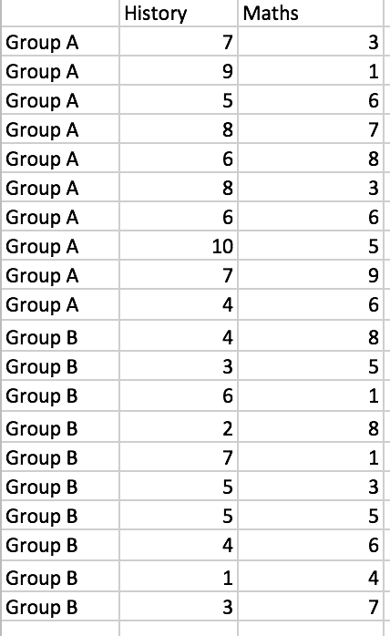
Here we have one factor, music, with 2 levels. This factor is going to affect our two dependent variables, i.e., the test scores of maths and history. Denoting this information in terms of variables, we can say that we have L = 2 (2 different music treatment groups) and P = 2 (maths and history scores).

A MANOVA test also takes into consideration a null hypothesis and an alternate hypothesis.:

 

The Calculations of MANOVA are too complex for this article so if you want to further read about it, check this paper. We will implement MANOVA in Excel using the ‘RealStats’ Add-ins. It can be downloaded from here.

Steps to perform MANOVA in Excel 2013:

Step 1: Download the ‘RealStats’ add-in from the link mentioned above

Step 2: Press “control+m” to open RealStats window

Step 3: Select “Analysis of variance”

Step 4: Select “MANOVA: single factor”

Step 5: Type an Input Range into the Input Range box. For example, if your data is in cells A1 to A25, type “A1:A25” into the Input Range box. Make sure you include all of your data, including headers and group names.

Step 6: Select “Significance analysis”, “Group Means” and “Multiple Anova”.

Step 7: Select an Output Range.

Step 8: Select an alpha level. In most cases, an alpha level of 0.05 (5 percent) works for most tests.

Step 9: Click “OK” to run. The data will be returned in your specified output range.

Step 10: Read the results. To figure out if you are going to reject the null hypothesis or not, you’ll basically be looking at two factors:

1. If the F-value (F)is larger than the f critical value (F crit)
2. If the p-value is smaller than your chosen alpha level.

And you are done!

 

RealStats add-on shows us the results by different methods. Each one of them denotes the same p-value. As the p-value is less than the alpha value, we will reject the null hypothesis. Or in simpler terms, it means that the music treatment did have a significant effect on the test results of students.

But we still cannot tell which subject was affected by the treatment and which was not. This is one of the limitations of MANOVA; even if it tells us whether the effect of a factor on a population was significant or not, it does not tell us which dependent variable was actually affected by the factor introduced.

For this purpose, we will see the “Multiple ANOVA” table to generate a helpful summary about it. The result will look like this:

 

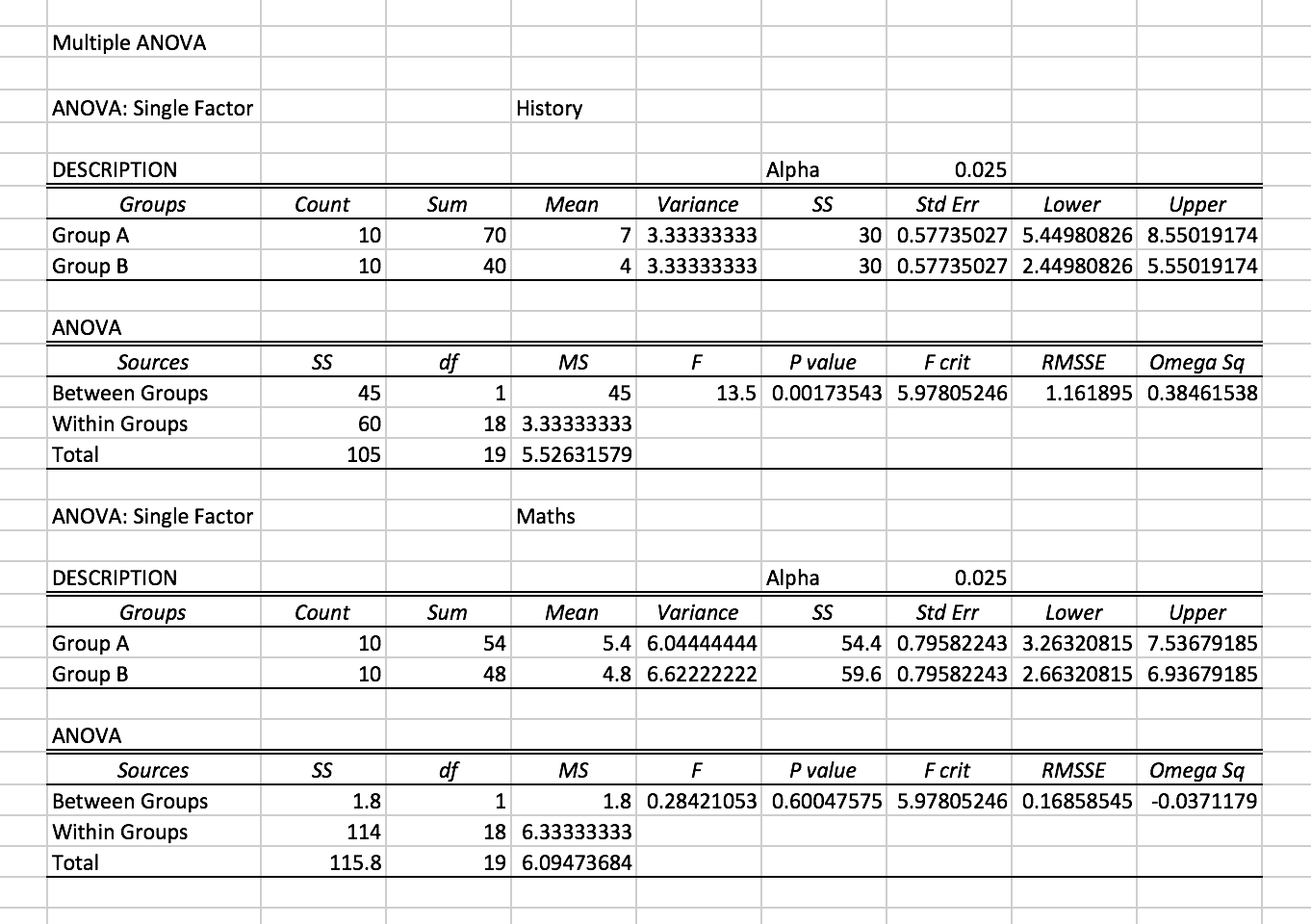
Here, we can see that the P value for history lies in a significant region (since P value less than 0.025) while for maths it does not. This means that the music treatment had a significant effect in improving the performance of students in history but did not have any significant effect in improving their performance in maths.

Based on this, we might consider picking and choosing subjects where this music approach can be used.

 

End Notes

I hope this article was helpful and now you’d be comfortable in solving similar problems using Analysis of Variance. I suggest you take different kinds of problem statements and take your time to solve them using the above-mentioned techniques.

You should also check out the below two resources to give your data science journey a huge boost:

• Introduction to Data Science Course
• Certified Program: Data Science for Beginners (with Interviews)

Did you find this article helpful? Please share your opinions / thoughts in the comments section below.

Learn, engage , hack and get hired!