A Detailed Guide to 7 Loss Functions for Machine Learning Algorithms with Python Code
Overview
- What are loss functions? And how do they work in machine learning algorithms? Find out in this article
- Loss functions are actually at the heart of these techniques that we regularly use
- This article covers multiple loss functions, where they work, and how you can code them in Python
Introduction
Picture this – you’ve trained a machine learning model on a given dataset and are ready to put it in front of your client. But how can you be sure that this model will give the optimum result? Is there a metric or a technique that will help you quickly evaluate your model on the dataset?
Yes – and that, in a nutshell, is where loss functions come into play in machine learning.
Loss functions are at the heart of the machine learning algorithms we love to use. But I’ve seen the majority of beginners and enthusiasts become quite confused regarding how and where to use them.

They’re not difficult to understand and will enhance your understand of machine learning algorithms infinitely. So, what are loss functions and how can you grasp their meaning?
In this article, I will discuss 7 common loss functions used in machine learning and explain where each of them is used. We have a lot to cover in this article so let’s begin!
Loss functions are one part of the entire machine learning journey you will take. Here’s the perfect course to help you get started and make you industry-ready:
Table of Contents
- What are Loss Functions?
- Regression Loss Functions
- Squared Error Loss
- Absolute Error Loss
- Huber Loss
- Binary Classification Loss Functions
- Binary Cross-Entropy
- Hinge Loss
- Multi-class Classification Loss Functions
- Multi-class Cross Entropy Loss
- Kullback Leibler Divergence Loss
What are Loss Functions?
Let’s say you are on the top of a hill and need to climb down. How do you decide where to walk towards?

Here’s what I would do:
- Look around to see all the possible paths
- Reject the ones going up. This is because these paths would actually cost me more energy and make my task even more difficult
- Finally, take the path that I think has the most slope downhill
This intuition that I just judged my decisions against? This is exactly what a loss function provides.
A loss function maps decisions to their associated costs.
Deciding to go up the slope will cost us energy and time. Deciding to go down will benefit us. Therefore, it has a negative cost.
In supervised machine learning algorithms, we want to minimize the error for each training example during the learning process. This is done using some optimization strategies like gradient descent. And this error comes from the loss function.
What’s the Difference between a Loss Function and a Cost Function?
I want to emphasize this here – although cost function and loss function are synonymous and used interchangeably, they are different.
A loss function is for a single training example. It is also sometimes called an error function. A cost function, on the other hand, is the average loss over the entire training dataset. The optimization strategies aim at minimizing the cost function.
Regression Loss Functions
You must be quite familiar with linear regression at this point. It deals with modeling a linear relationship between a dependent variable, Y, and several independent variables, X_i’s. Thus, we essentially fit a line in space on these variables.
Y = a0 + a1 * X1 + a2 * X2 + ....+ an * Xn
We will use the given data points to find the coefficients a0, a1, …, an.
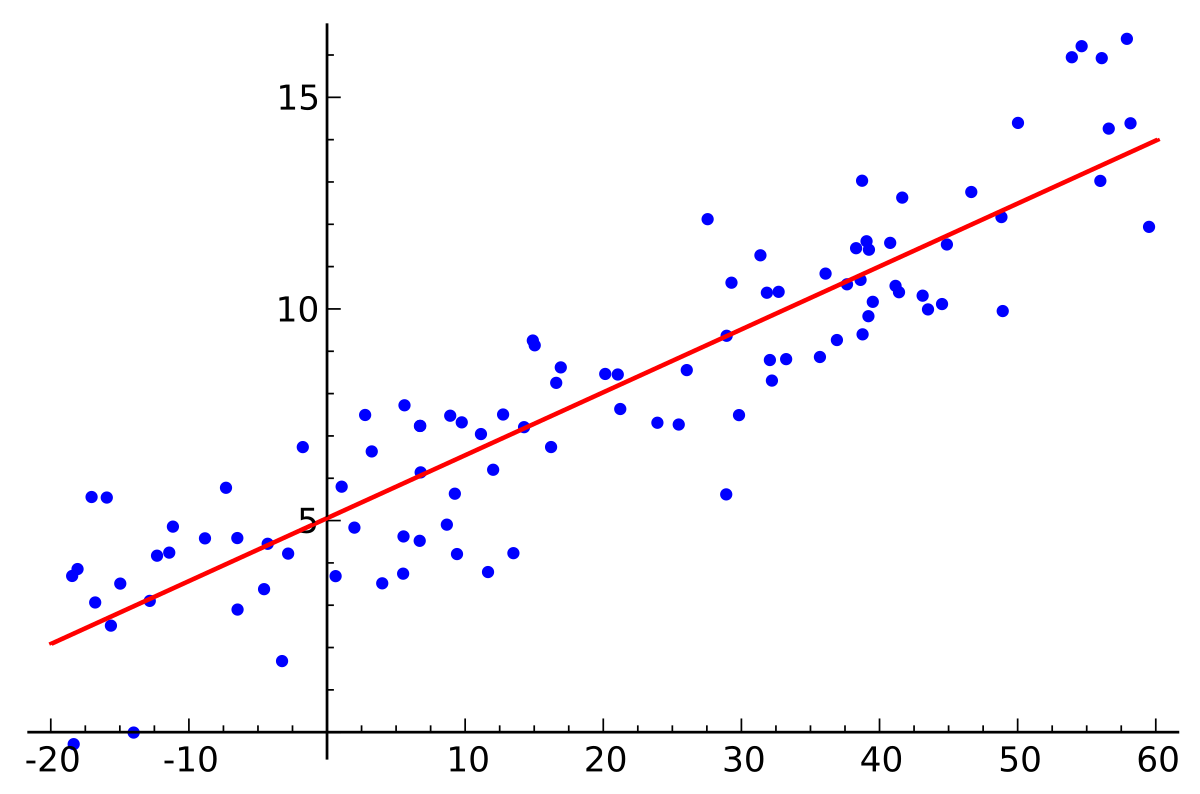
Source: Wikipedia
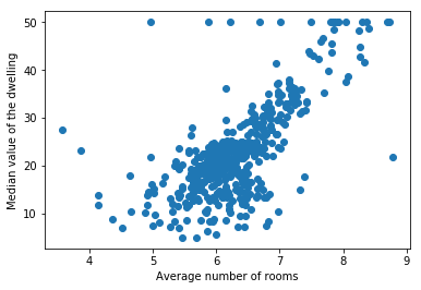
We will use the famous Boston Housing Dataset for understanding this concept. And to keep things simple, we will use only one feature – the Average number of rooms per dwelling (X) – to predict the dependent variable – Median Value (Y) of houses in $1000′ s.
We will use Gradient Descent as an optimization strategy to find the regression line. I will not go into the intricate details about Gradient Descent, but here is a reminder of the Weight Update Rule:
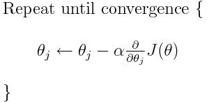
Source: Hackernoon.com
Here, theta_j is the weight to be updated, alpha is the learning rate and J is the cost function. The cost function is parameterized by theta. Our aim is to find the value of theta which yields minimum overall cost.
You can get an in-depth explanation of Gradient Descent and how it works here.
I have defined the steps that we will follow for each loss function below:
- Write the expression for our predictor function, f(X) and identify the parameters that we need to find
- Identify the loss to use for each training example
- Find the expression for the Cost Function – the average loss on all examples
- Find the gradient of the Cost Function with respect to each unknown parameter
- Decide on the learning rate and run the weight update rule for a fixed number of iterations
1. Squared Error Loss
Squared Error loss for each training example, also known as L2 Loss, is the square of the difference between the actual and the predicted values:
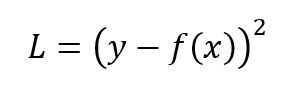
The corresponding cost function is the Mean of these Squared Errors (MSE).
I encourage you to try and find the gradient for gradient descent yourself before referring to the code below.
I used this code on the Boston data for different values of the learning rate for 500 iterations each:
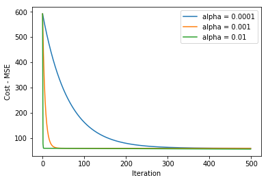
Here’s a task for you. Try running the code for a learning rate of 0.1 again for 500 iterations. Let me know your observations and any possible explanations in the comments section.
Let’s talk a bit more about the MSE loss function. It is a positive quadratic function (of the form ax^2 + bx + c where a > 0). Remember how it looks graphically?
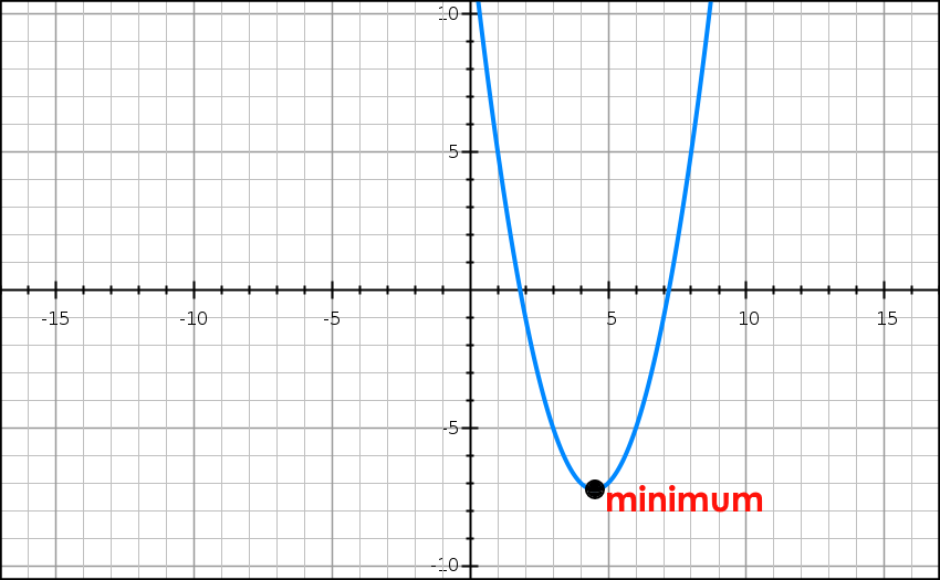
A quadratic function only has a global minimum. Since there are no local minima, we will never get stuck in one. Hence, it is always guaranteed that Gradient Descent will converge (if it converges at all) to the global minimum.
The MSE loss function penalizes the model for making large errors by squaring them. Squaring a large quantity makes it even larger, right? But there’s a caveat. This property makes the MSE cost function less robust to outliers. Therefore, it should not be used if our data is prone to many outliers.
2. Absolute Error Loss
Absolute Error for each training example is the distance between the predicted and the actual values, irrespective of the sign. Absolute Error is also known as the L1 loss:
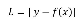
As I mentioned before, the cost is the Mean of these Absolute Errors (MAE).
The MAE cost is more robust to outliers as compared to MSE. However, handling the absolute or modulus operator in mathematical equations is not easy. I’m sure a lot of you must agree with this! We can consider this as a disadvantage of MAE.
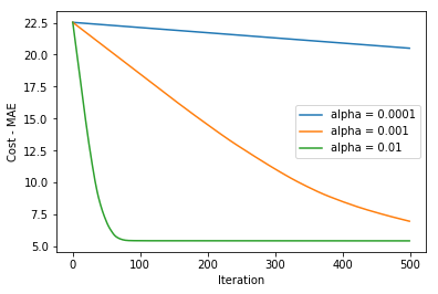
Here is the code for the update_weight function with MAE cost:
We get the below plot after running the code for 500 iterations with different learning rates:
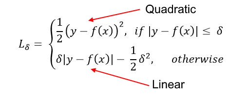
3. Huber Loss
The Huber loss combines the best properties of MSE and MAE. It is quadratic for smaller errors and is linear otherwise (and similarly for its gradient). It is identified by its delta parameter:
We obtain the below plot for 500 iterations of weight update at a learning rate of 0.0001 for different values of the delta parameter: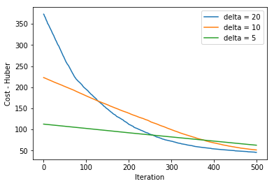
Huber loss is more robust to outliers than MSE. It is used in Robust Regression, M-estimation and Additive Modelling. A variant of Huber Loss is also used in classification.
Binary Classification Loss Functions
The name is pretty self-explanatory. Binary Classification refers to assigning an object into one of two classes. This classification is based on a rule applied to the input feature vector. For example, classifying an email as spam or not spam based on, say its subject line, is binary classification.
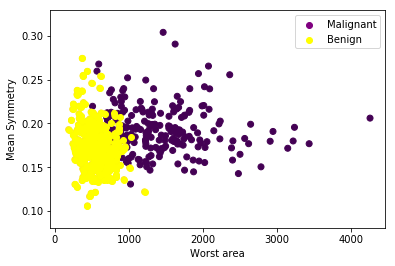
I will illustrate these binary classification loss functions on the Breast Cancer dataset.
We want to classify a tumor as ‘Malignant’ or ‘Benign’ based on features like average radius, area, perimeter, etc. For simplification, we will use only two input features (X_1 and X_2) namely ‘worst area’ and ‘mean symmetry’ for classification. The target value Y can be 0 (Malignant) or 1 (Benign).
Here is a scatter plot for our data:
1. Binary Cross Entropy Loss
Let us start by understanding the term ‘entropy’. Generally, we use entropy to indicate disorder or uncertainty. It is measured for a random variable X with probability distribution p(X):
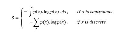
The negative sign is used to make the overall quantity positive.
A greater value of entropy for a probability distribution indicates a greater uncertainty in the distribution. Likewise, a smaller value indicates a more certain distribution.
This makes binary cross-entropy suitable as a loss function – you want to minimize its value. We use binary cross-entropy loss for classification models which output a probability p.
Probability that the element belongs to class 1 (or positive class) = p
Then, the probability that the element belongs to class 0 (or negative class) = 1 - p
Then, the cross-entropy loss for output label y (can take values 0 and 1) and predicted probability p is defined as:
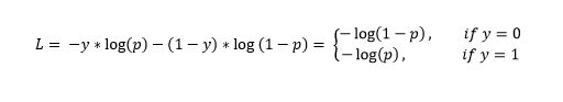
This is also called Log-Loss. To calculate the probability p, we can use the sigmoid function. Here, z is a function of our input features:
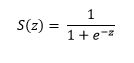
The range of the sigmoid function is [0, 1] which makes it suitable for calculating probability.
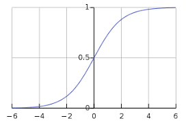
Try to find the gradient yourself and then look at the code for the update_weight function below.
I got the below plot on using the weight update rule for 1000 iterations with different values of alpha:
2. Hinge Loss
Hinge loss is primarily used with Support Vector Machine (SVM) Classifiers with class labels -1 and 1. So make sure you change the label of the ‘Malignant’ class in the dataset from 0 to -1.
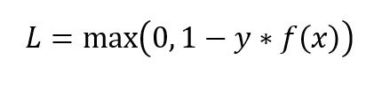
Hinge Loss not only penalizes the wrong predictions but also the right predictions that are not confident.
Hinge loss for an input-output pair (x, y) is given as:
After running the update function for 2000 iterations with three different values of alpha, we obtain this plot:
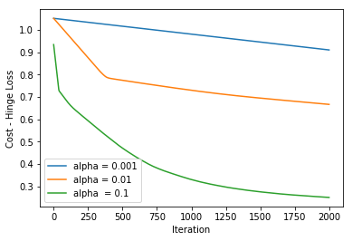
Hinge Loss simplifies the mathematics for SVM while maximizing the loss (as compared to Log-Loss). It is used when we want to make real-time decisions with not a laser-sharp focus on accuracy.
Multi-Class Classification Loss Functions
Emails are not just classified as spam or not spam (this isn’t the 90s anymore!). They are classified into various other categories – Work, Home, Social, Promotions, etc. This is a Multi-Class Classification use case.
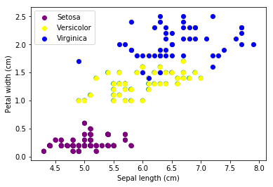
We’ll use the Iris Dataset for understanding the remaining two loss functions. We will use 2 features X_1, Sepal length and feature X_2, Petal width, to predict the class (Y) of the Iris flower – Setosa, Versicolor or Virginica
Our task is to implement the classifier using a neural network model and the in-built Adam optimizer in Keras. This is because as the number of parameters increases, the math, as well as the code, will become difficult to comprehend.
If you are new to Neural Networks, I highly recommend reading this article first.
Here is the scatter plot for our data:
1. Multi-Class Cross Entropy Loss
The multi-class cross-entropy loss is a generalization of the Binary Cross Entropy loss. The loss for input vector X_i and the corresponding one-hot encoded target vector Y_i is:
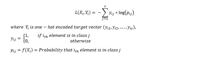
We use the softmax function to find the probabilities p_ij:
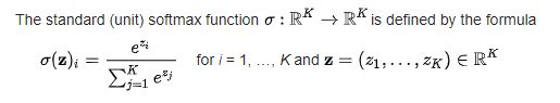
Source: Wikipedia
“Softmax is implemented through a neural network layer just before the output layer. The Softmax layer must have the same number of nodes as the output layer.” Google Developer’s Blog
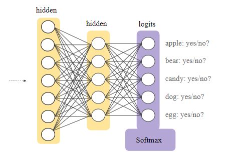
Finally, our output is the class with the maximum probability for the given input.
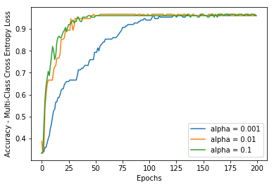
We build a model using an input layer and an output layer and compile it with different learning rates. Specify the loss parameter as ‘categorical_crossentropy’ in the model.compile() statement:
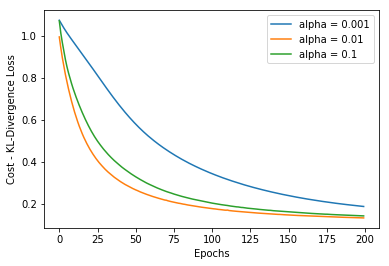
Here are the plots for cost and accuracy respectively after training for 200 epochs:

2. KL-Divergence
The Kullback-Liebler Divergence is a measure of how a probability distribution differs from another distribution. A KL-divergence of zero indicates that the distributions are identical.
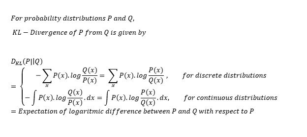
Notice that the divergence function is not symmetric.
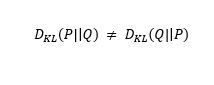
This is why KL-Divergence cannot be used as a distance metric.
I will describe the basic approach of using KL-Divergence as a loss function without getting into its math. We want to approximate the true probability distribution P of our target variables with respect to the input features, given some approximate distribution Q. Since KL-Divergence is not symmetric, we can do this in two ways:
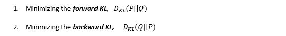
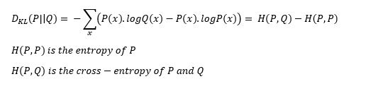
The first approach is used in Supervised learning, the second in Reinforcement Learning. KL-Divergence is functionally similar to multi-class cross-entropy and is also called relative entropy of P with respect to Q:
We specify the ‘kullback_leibler_divergence’ as the value of the loss parameter in the compile() function as we did before with the multi-class cross-entropy loss.

KL-Divergence is used more commonly to approximate complex functions than in multi-class classification. We come across KL-Divergence frequently while playing with deep-generative models like Variational Autoencoders (VAEs).
End Notes
Woah! We have covered a lot of ground here. Give yourself a pat on your back for making it all the way to the end. This was quite a comprehensive list of loss functions we typically use in machine learning.
I would suggest going through this article a couple of times more as you proceed with your machine learning journey. This isn’t a one-time effort. It will take a few readings and experience to understand how and where these loss functions work.
Make sure to experiment with these loss functions and let me know your observations down in the comments. Also, let me know other topics that you would like to read about. I will do my best to cover them in future articles.
Meanwhile, make sure you check out our comprehensive beginner-level machine learning course:


Thank you very much for the article. Excellent and detailed explanatins. Any idea on how to use Machine Learning for studying the lotteries? Not to play the lotteries, but to study some behaviours based on data gathered as a time series.
Hi Joe, Thank you for your appreciation. Regarding the lotteries problem, please define your problem statement clearly. We have covered Time-Series Analysis in a vast array of articles. I recommend you go through them according to your needs. I would suggest you also use our discussion forum for the same. You will be guided by experts all over the world. All the best!
Great article, I can see incorporating some of these in our current projects and will introduce our lunch and learn team to your article. Thank you for taking the time to write it!
Thank you for your appreciation, Michael!
It was such a wonderful article!! Thanks for sharing mate!
Great Article.. Thank you so much!! By the way.. do you have something to share about “ The quantification of certainty above reasonable doubt in the judgment of the merits of criminal proceedings by artificial intelligence “
Great article, complete with code. Any idea on how to create your own custom loss function?