Overview

• Did you know you can work with image data using machine learning techniques?
• Deep learning models are the flavor of the month, but not everyone has access to unlimited resources – that’s where machine learning comes to the rescue!
• Learn how to extract features from images using Python in this article

 

Introduction

Have you worked with image data before? Perhaps you’ve wanted to build your own object detection model, or simply want to count the number of people walking into a building. The possibilities of working with images using computer vision techniques are endless.

But I’ve seen a trend among data scientists recently. There’s a strong belief that when it comes to working with unstructured data, especially image data, deep learning models are the way forward. Deep learning techniques undoubtedly perform extremely well, but is that the only way to work with images?

Not all of us have unlimited resources like the big technology behemoths such as Google and Facebook. So how can we work with image data if not through the lens of deep learning?

We can leverage the power of machine learning! That’s right – we can use simple machine learning models like decision trees or Support Vector Machines (SVM). If we provide the right data and features, these machine learning models can perform adequately and can even be used as a benchmark solution.

So in this beginner-friendly article, we will understand the different ways in which we can generate features from images. You can then use these methods in your favorite machine learning algorithms!

 

Table of Contents

1. How do Machines Store Images?
2. Reading Image Data in Python
3. Method #1 for Feature Extraction from Image Data: Grayscale Pixel Values as Features
4. Method #2 for Feature Extraction from Image Data: Mean Pixel Value of Channels
5. Method #3 for Feature Extraction from Image Data: Extracting Edges

 

How do Machines Store Images?

Let’s start with the basics. It’s important to understand how we can read and store images on our machines before we look at anything else. Consider this the ‘pd.read_‘ function, but for images.

I’ll kick things off with a simple example. Look at the image below:

We have an image of the number 8. Look really closely at the image – you’ll notice that it is made up of small square boxes. These are called pixels.

There is a caveat, however. We see the images as they are – in their visual form. We can easily differentiate the edges and colors to identify what is in the picture. Machines, on the other hand, struggle to do this. They store images in the form of numbers. Have a look at the image below:

Machines store images in the form of a matrix of numbers. The size of this matrix depends on the number of pixels we have in any given image.

Let’s say the dimensions of an image are 180 x 200 or n x m. These dimensions are basically the number of pixels in the image (height x width).

These numbers, or the pixel values, denote the intensity or brightness of the pixel. Smaller numbers (closer to zero) represent black, and larger numbers (closer to 255) denote white. You’ll understand whatever we have learned so far by analyzing the below image.

The dimensions of the below image are 22 x 16, which you can verify by counting the number of pixels:

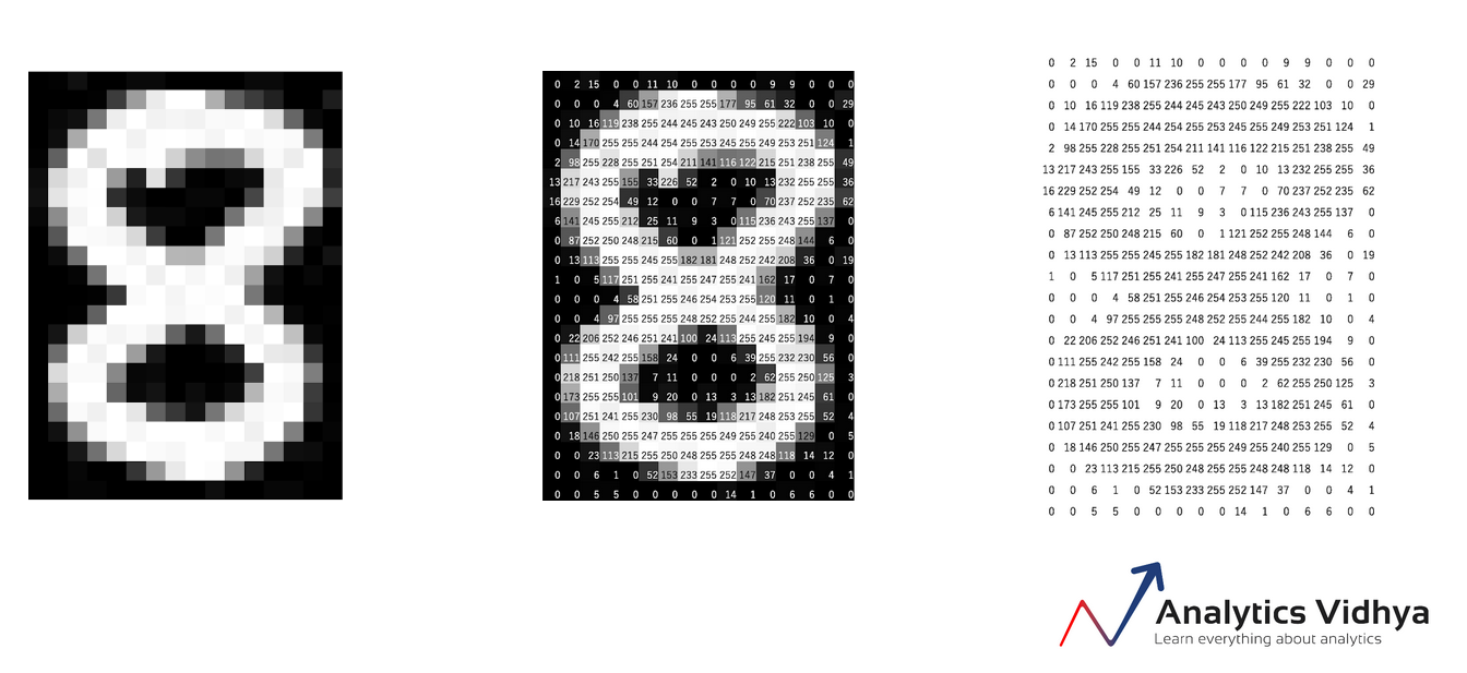
Source: Applied Machine Learning Course

The example we just discussed is that of a black and white image. What about colored images (which are far more prevalent in the real world)? Do you think colored images also stored in the form of a 2D matrix as well?

A colored image is typically composed of multiple colors and almost all colors can be generated from three primary colors – red, green and blue.

Hence, in the case of a colored image, there are three Matrices (or channels) – Red, Green, and Blue. Each matrix has values between 0-255 representing the intensity of the color for that pixel. Consider the below image to understand this concept:

Source: Applied Machine Learning Course

We have a colored image on the left (as we humans would see it). On the right, we have three matrices for the three color channels – Red, Green, and Blue. The three channels are superimposed to form a colored image.

Note that these are not the original pixel values for the given image as the original matrix would be very large and difficult to visualize. Also, there are various other formats in which the images are stored. RGB is the most popular one and hence I have addressed it here. You can read more about the other popular formats here.

 

Reading Image Data in Python

Let’s put our theoretical knowledge into practice. We’ll fire up Python and load an image to see what the matrix looks like:

(28,28)

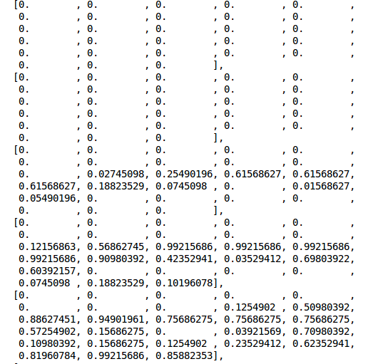
The matrix has 784 values and this is a very small part of the complete matrix. Here’s a LIVE coding window for you to run all the above code and see the result without leaving this article! Go ahead and play around with it:

Let’s now dive into the core idea behind this article and explore various methods of using pixel values as features.

 

Method #1: Grayscale Pixel Values as Features

The simplest way to create features from an image is to use these raw pixel values as separate features.

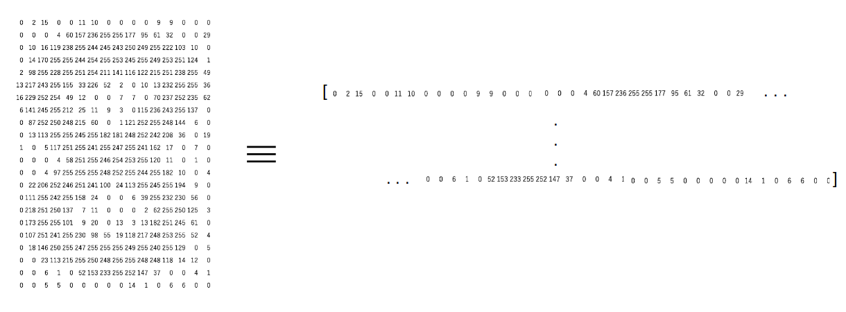
Consider the same example for our image above (the number ‘8’) – the dimension of the image is 28 x 28.

Can you guess the number of features for this image? The number of features will be the same as the number of pixels! Hence, that number will be 784.

Now here’s another curious question – how do we arrange these 784 pixels as features? Well, we can simply append every pixel value one after the other to generate a feature vector. This is illustrated in the image below:

Let us take an image in Python and create these features for that image:

(650, 450

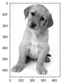
The image shape here is 650 x 450. Hence, the number of features should be 297,000. We can generate this using the reshape function from NumPy where we specify the dimension of the image:

(297000,)
array([0.96470588, 0.96470588, 0.96470588, ..., 0.96862745, 0.96470588,
       0.96470588])

Here, we have our feature – which is a 1D array of length 297,000. Easy, right? Try your hand at this feature extraction method in the below live coding window:

But here, we only had a single channel or a grayscale image. Can we do the same for a colored image? Let’s find out!

 

Method #2: Mean Pixel Value of Channels

While reading the image in the previous section, we had set the parameter ‘as_gray = True’. So we only had one channel in the image and we could easily append the pixel values. Let us remove the parameter and load the image again:

(660, 450, 3)

This time, the image has a dimension (660, 450, 3), where 3 is the number of channels. We can go ahead and create the features as we did previously. The number of features, in this case, will be 660*450*3 = 891,000.

Alternatively, here is another approach we can use:

Instead of using the pixel values from the three channels separately, we can generate a new matrix that has the mean value of pixels from all three channels.

The image below will give you even more clarity around this idea: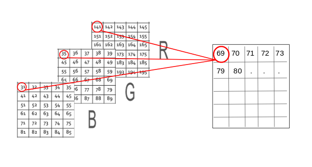

By doing so, the number of features remains the same and we also take into account the pixel values from all three channels of the image. Let us code this out in Python. We will create a new matrix with the same size 660 x 450, where all values are initialized to 0. This matrix will store the mean pixel values for the three channels:

(660, 450)

We have a 3D matrix of dimension (660 x 450 x 3) where 660 is the height, 450 is the width and 3 is the number of channels. To get the average pixel values, we will use a for loop:

The new matrix will have the same height and width but only 1 channel. Now we can follow the same steps that we did in the previous section. We append the pixel values one after the other to get a 1D array:

(297000,)

Method #3: Extracting Edge Features

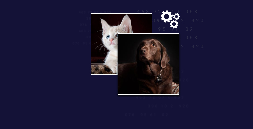
Consider that we are given the below image and we need to identify the objects present in it:

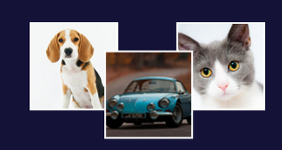
You must have recognized the objects in an instant – a dog, a car and a cat. What are the features that you considered while differentiating each of these images? The shape could be one important factor, followed by color, or size. What if the machine could also identify the shape as we do?

A similar idea is to extract edges as features and use that as the input for the model. I want you to think about this for a moment – how can we identify edges in an image? Edge is basically where there is a sharp change in color. Look at the below image:

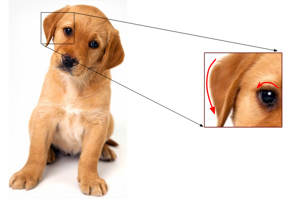
I have highlighted two edges here. We could identify the edge because there was a change in color from white to brown (in the right image) and brown to black (in the left). And as we know, an image is represented in the form of numbers. So, we will look for pixels around which there is a drastic change in the pixel values.

Let’s say we have the following matrix for the image:

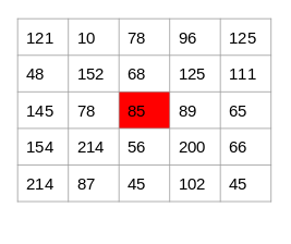
Source: Applied Machine Learning Course

To identify if a pixel is an edge or not, we will simply subtract the values on either side of the pixel. For this example, we have the highlighted value of 85. We will find the difference between the values 89 and 78. Since this difference is not very large, we can say that there is no edge around this pixel.

Now consider the pixel 125 highlighted in the below image:

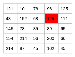
Source: Applied Machine Learning Course

Since the difference between the values on either side of this pixel is large, we can conclude that there is a significant transition at this pixel and hence it is an edge. Now the question is, do we have to do this step manually?

No! There are various kernels that can be used to highlight the edges in an image. The method we just discussed can also be achieved using the Prewitt kernel (in the x-direction). Given below is the Prewitt kernel:

We take the values surrounding the selected pixel and multiply it with the selected kernel (Prewitt kernel). We can then add the resulting values to get a final value. Since we already have -1 in one column and 1 in the other column, adding the values is equivalent to taking the difference.

There are various other kernels and I have mentioned four most popularly used ones below:

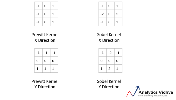
Source: Applied Machine Learning Course

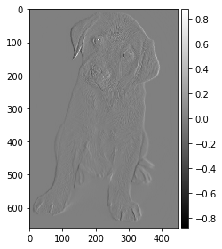
Let’s now go back to the notebook and generate edge features for the same image:

 

End Notes

This was a friendly introduction to getting your hands dirty with image data. I feel this is a very important part of a data scientist’s toolkit given the rapid rise in the number of images being generated these days.

So what can you do once you are acquainted with this topic? We will deep dive into the next steps in my next article – dropping soon! So watch this space and if you have any questions or thoughts on this article, let me know in the comments section below.

Edit: Here is an article on advanced feature Extraction Techniques for Images

• Feature Engineering for Images: A Valuable Introduction to the HOG Feature Descriptor

Also, here are two comprehensive courses to get you started with machine learning and deep learning:

• Applied Machine Learning: Beginner to Professional
• Computer Vision using Deep Learning