An End-to-End Guide to Understand the Math behind XGBoost
Introduction
Ever since its introduction in 2014, XGBoost has been lauded as the holy grail of machine learning hackathons and competitions. From predicting ad click-through rates to classifying high energy physics events, XGBoost has proved its mettle in terms of performance – and speed.
I always turn to XGBoost as my first algorithm of choice in any ML hackathon. The accuracy it consistently gives, and the time it saves, demonstrates how useful it is. But how does it actually work? What kind of mathematics power XGBoost? We’ll figure out the answers to these questions soon.

Tianqi Chen, one of the co-creators of XGBoost, announced (in 2016) that the innovative system features and algorithmic optimizations in XGBoost have rendered it 10 times faster than most sought after machine learning solutions. A truly amazing technique!
In this article, we will first look at the power of XGBoost, and then deep dive into the inner workings of this popular and powerful technique. It’s good to be able to implement it in Python or R, but understanding the nitty-gritties of the algorithm will help you become a better data scientist.
Note:
We recommend going through the below article as well to fully understand the various terms and concepts mentioned in this article:
If you prefer to learn the same concepts in the form of a structured course, you can enrol in this free course as well:
Table of Contents
- The Power of XGBoost
- Why Ensemble Learning?
- Bagging
- Boosting
- Demonstrating the Potential of Boosting
- Using gradient descent for optimizing the loss function
- Unique Features of XGBoost
The Power of XGBoost
The beauty of this powerful algorithm lies in its scalability, which drives fast learning through parallel and distributed computing and offers efficient memory usage.
It’s no wonder then that CERN recognized it as the best approach to classify signals from the Large Hadron Collider. This particular challenge posed by CERN required a solution that would be scalable to process data being generated at the rate of 3 petabytes per year and effectively distinguish an extremely rare signal from background noises in a complex physical process. XGBoost emerged as the most useful, straightforward and robust solution.
Now, let’s deep dive into the inner workings of XGBoost.
Why ensemble learning?
XGBoost is an ensemble learning method. Sometimes, it may not be sufficient to rely upon the results of just one machine learning model. Ensemble learning offers a systematic solution to combine the predictive power of multiple learners. The resultant is a single model which gives the aggregated output from several models.
The models that form the ensemble, also known as base learners, could be either from the same learning algorithm or different learning algorithms. Bagging and boosting are two widely used ensemble learners. Though these two techniques can be used with several statistical models, the most predominant usage has been with decision trees.
Let’s briefly discuss bagging before taking a more detailed look at the concept of boosting.
Bagging
While decision trees are one of the most easily interpretable models, they exhibit highly variable behavior. Consider a single training dataset that we randomly split into two parts. Now, let’s use each part to train a decision tree in order to obtain two models.
When we fit both these models, they would yield different results. Decision trees are said to be associated with high variance due to this behavior. Bagging or boosting aggregation helps to reduce the variance in any learner. Several decision trees which are generated in parallel, form the base learners of bagging technique. Data sampled with replacement is fed to these learners for training. The final prediction is the averaged output from all the learners.
Boosting
In boosting, the trees are built sequentially such that each subsequent tree aims to reduce the errors of the previous tree. Each tree learns from its predecessors and updates the residual errors. Hence, the tree that grows next in the sequence will learn from an updated version of the residuals.
The base learners in boosting are weak learners in which the bias is high, and the predictive power is just a tad better than random guessing. Each of these weak learners contributes some vital information for prediction, enabling the boosting technique to produce a strong learner by effectively combining these weak learners. The final strong learner brings down both the bias and the variance.
In contrast to bagging techniques like Random Forest, in which trees are grown to their maximum extent, boosting makes use of trees with fewer splits. Such small trees, which are not very deep, are highly interpretable. Parameters like the number of trees or iterations, the rate at which the gradient boosting learns, and the depth of the tree, could be optimally selected through validation techniques like k-fold cross validation. Having a large number of trees might lead to overfitting. So, it is necessary to carefully choose the stopping criteria for boosting.
The boosting ensemble technique consists of three simple steps:
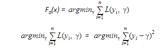
- An initial model F0 is defined to predict the target variable y. This model will be associated with a residual (y – F0)
- A new model h1 is fit to the residuals from the previous step
- Now, F0 and h1 are combined to give F1, the boosted version of F0. The mean squared error from F1 will be lower than that from F0:
![]()
To improve the performance of F1, we could model after the residuals of F1 and create a new model F2:
![]()
This can be done for ‘m’ iterations, until residuals have been minimized as much as possible:
![]()
Here, the additive learners do not disturb the functions created in the previous steps. Instead, they impart information of their own to bring down the errors.
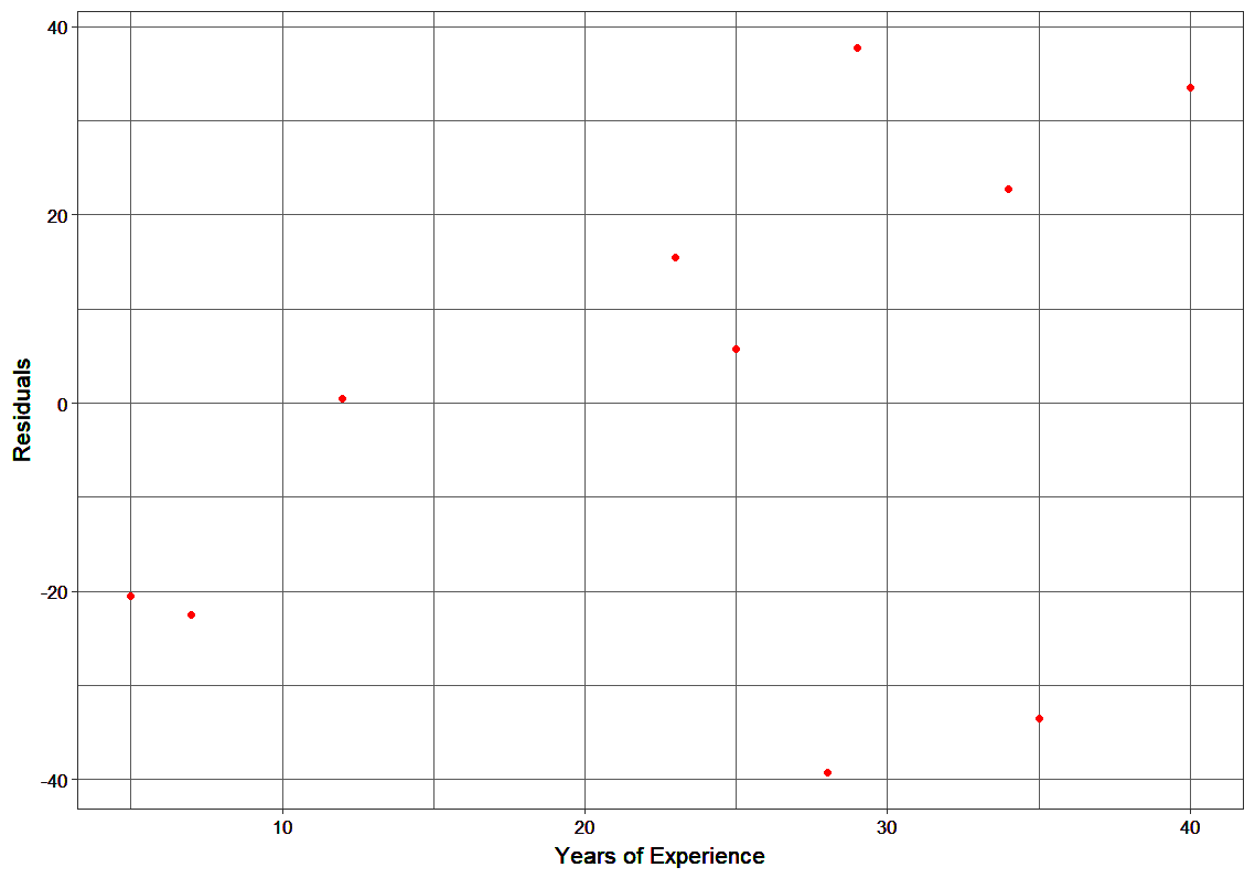
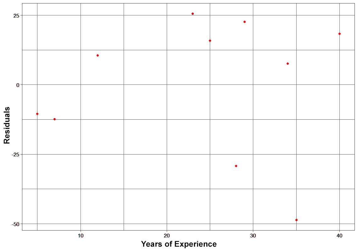
Demonstrating the Potential of Boosting
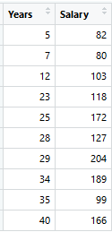
Consider the following data where the years of experience is predictor variable and salary (in thousand dollars) is the target. Using regression trees as base learners, we can create an ensemble model to predict the salary. For the sake of simplicity, we can choose square loss as our loss function and our objective would be to minimize the square error.
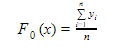
As the first step, the model should be initialized with a function F0(x). F0(x) should be a function which minimizes the loss function or MSE (mean squared error), in this case:
Taking the first differential of the above equation with respect to γ, it is seen that the function minimizes at the mean i=1nyin. So, the boosting model could be initiated with:
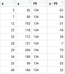
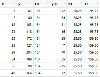
F0(x) gives the predictions from the first stage of our model. Now, the residual error for each instance is (yi – F0(x)).
We can use the residuals from F0(x) to create h1(x). h1(x) will be a regression tree which will try and reduce the residuals from the previous step. The output of h1(x) won’t be a prediction of y; instead, it will help in predicting the successive function F1(x) which will bring down the residuals.
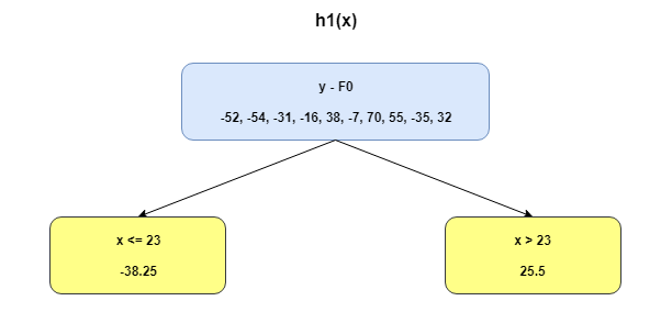
The additive model h1(x) computes the mean of the residuals (y – F0) at each leaf of the tree. The boosted function F1(x) is obtained by summing F0(x) and h1(x). This way h1(x) learns from the residuals of F0(x) and suppresses it in F1(x).
This can be repeated for 2 more iterations to compute h2(x) and h3(x). Each of these additive learners, hm(x), will make use of the residuals from the preceding function, Fm-1(x).
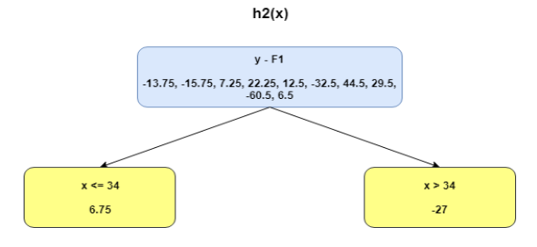
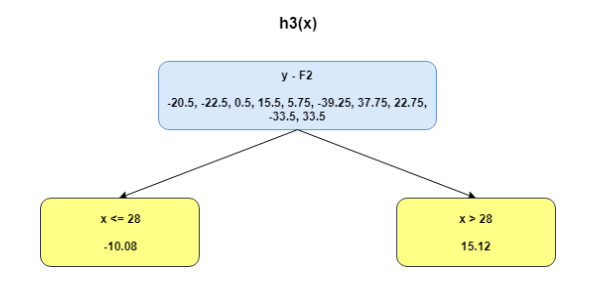
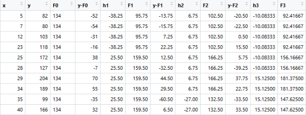
The MSEs for F0(x), F1(x) and F2(x) are 875, 692 and 540. It’s amazing how these simple weak learners can bring about a huge reduction in error!
Note that each learner, hm(x), is trained on the residuals. All the additive learners in boosting are modeled after the residual errors at each step. Intuitively, it could be observed that the boosting learners make use of the patterns in residual errors. At the stage where maximum accuracy is reached by boosting, the residuals appear to be randomly distributed without any pattern.
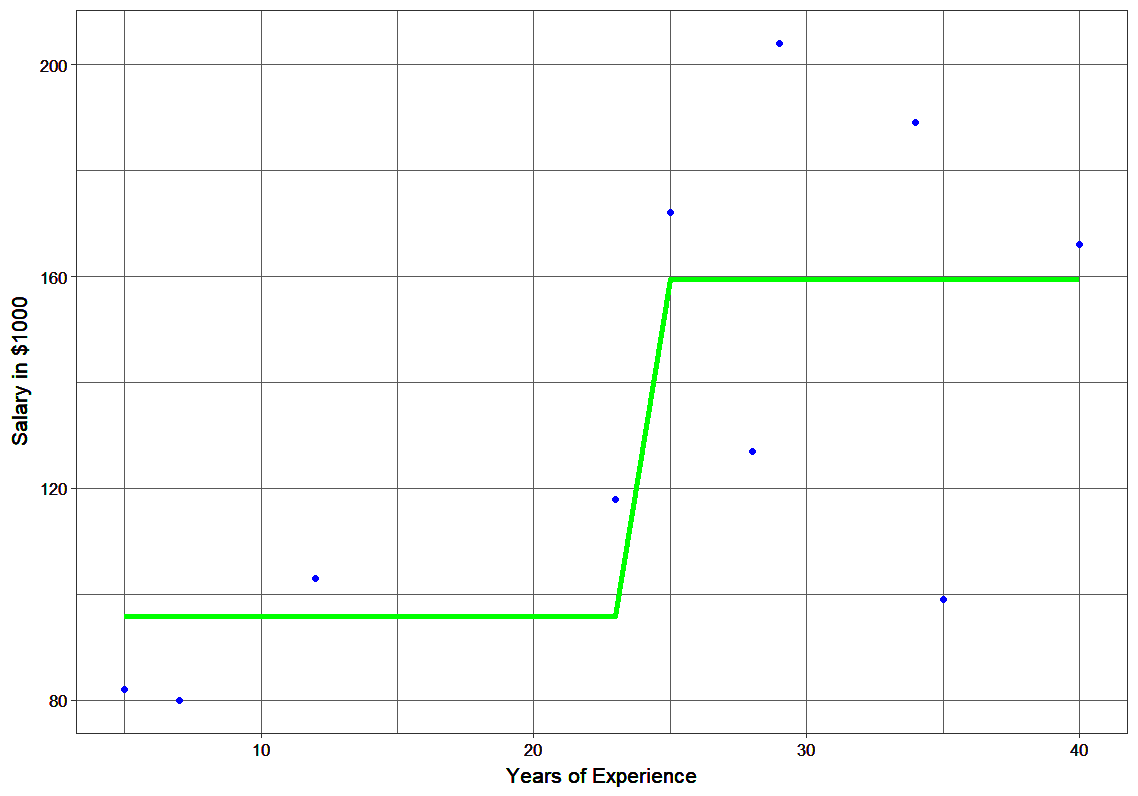
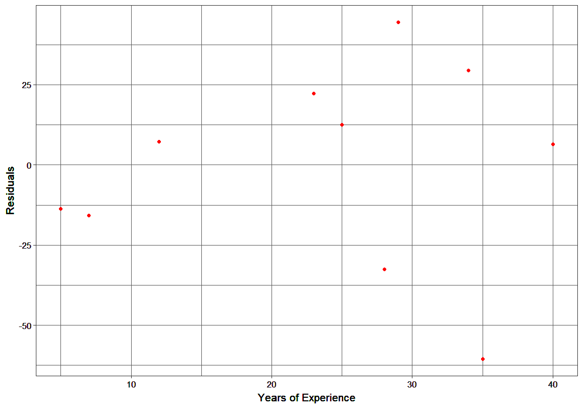
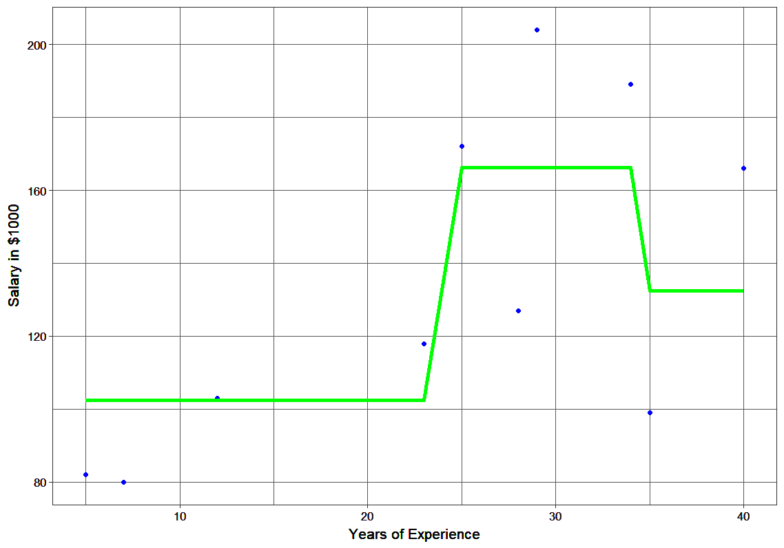
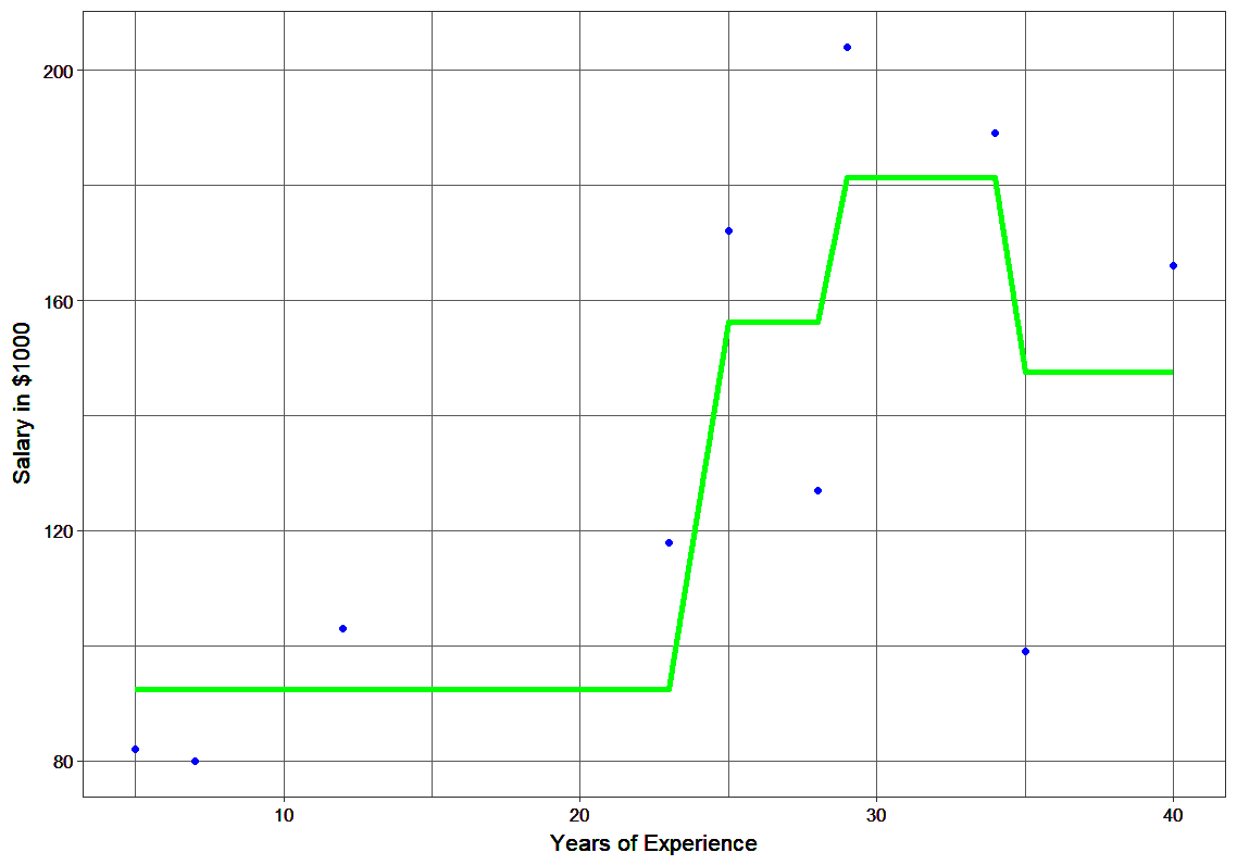
Plots of Fn and hn
Using gradient descent for optimizing the loss function
In the case discussed above, MSE was the loss function. The mean minimized the error here. When MAE (mean absolute error) is the loss function, the median would be used as F0(x) to initialize the model. A unit change in y would cause a unit change in MAE as well.
For MSE, the change observed would be roughly exponential. Instead of fitting hm(x) on the residuals, fitting it on the gradient of loss function, or the step along which loss occurs, would make this process generic and applicable across all loss functions.
Gradient descent helps us minimize any differentiable function. Earlier, the regression tree for hm(x) predicted the mean residual at each terminal node of the tree. In gradient boosting, the average gradient component would be computed.
For each node, there is a factor γ with which hm(x) is multiplied. This accounts for the difference in impact of each branch of the split. Gradient boosting helps in predicting the optimal gradient for the additive model, unlike classical gradient descent techniques which reduce error in the output at each iteration.
The following steps are involved in gradient boosting:
- F0(x) – with which we initialize the boosting algorithm – is to be defined:
![]()
- The gradient of the loss function is computed iteratively:
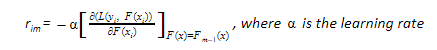
- Each hm(x) is fit on the gradient obtained at each step
- The multiplicative factor γm for each terminal node is derived and the boosted model Fm(x) is defined:
![]()
Unique features of XGBoost
XGBoost is a popular implementation of gradient boosting. Let’s discuss some features of XGBoost that make it so interesting.
- Regularization: XGBoost has an option to penalize complex models through both L1 and L2 regularization. Regularization helps in preventing overfitting
- Handling sparse data: Missing values or data processing steps like one-hot encoding make data sparse. XGBoost incorporates a sparsity-aware split finding algorithm to handle different types of sparsity patterns in the data
- Weighted quantile sketch: Most existing tree based algorithms can find the split points when the data points are of equal weights (using quantile sketch algorithm). However, they are not equipped to handle weighted data. XGBoost has a distributed weighted quantile sketch algorithm to effectively handle weighted data
- Block structure for parallel learning: For faster computing, XGBoost can make use of multiple cores on the CPU. This is possible because of a block structure in its system design. Data is sorted and stored in in-memory units called blocks. Unlike other algorithms, this enables the data layout to be reused by subsequent iterations, instead of computing it again. This feature also serves useful for steps like split finding and column sub-sampling
- Cache awareness: In XGBoost, non-continuous memory access is required to get the gradient statistics by row index. Hence, XGBoost has been designed to make optimal use of hardware. This is done by allocating internal buffers in each thread, where the gradient statistics can be stored
- Out-of-core computing: This feature optimizes the available disk space and maximizes its usage when handling huge datasets that do not fit into memory
Python Code for XGBoost
Here’s a live coding window to see how XGBoost works and play around with the code without leaving this article!
End Notes
So that was all about the mathematics that power the popular XGBoost algorithm. If your basics are solid, this article must have been a breeze for you. It’s such a powerful algorithm and while there are other techniques that have spawned from it (like CATBoost), XGBoost remains a game changer in the machine learning community.
I would highly recommend you to take up this course to sharpen your skills in machine learning and learn all the state-of-the-art techniques used in the field
If you have any feedback on the article, or questions on any of the above concepts, connect with me in the comments section below.
About the author

Ramya Bhaskar Sundaram – Data Scientist, Noah Data
It’s safe to say my forte is advanced analytics. The charm and magnificence of statistics have enticed me, all through my journey as a Data Scientist. There is a definite beauty in how the simplest of statistical techniques can bring out the most intriguing insights from data. My fascination for statistics has helped me to continuously learn and expand my skill set in the domain.My experience spans across multiple verticals: Renewable Energy, Semiconductor, Financial Technology, Educational Technology, E-Commerce Aggregator, Digital Marketing, CRM, Fabricated Metal Manufacturing, Human Resources.


Nice explanation !
Hi. Nice article. Thanks for sharing. Couple of clarification 1. what's the formula for calculating the h1(X) 2. How did the split happen x23.
Hi Srinivas, The split was decided based on a simple approach. A tree with a split at x = 23 returned the least SSE during prediction. Hope this answers your question. Thanks & Regards, Ramya Bhaskar
Do you have your app for iOS?
yes
Great article. Can you just give a brief in the terms of regularization. What parameters get regularized? How the regularization happens in the case of multiple trees?
Very enlightening about the concept and interesting read. Can you brief me about loss functions?
Thanks for sharing this great ariticle! Just have one clarification: h1 is calculated by some criterion(>23) on y-f0. In the resulted table, why there are some h1 with value 25.5 when y-f0 is negative (<23)?
Grate post! How this method treats outliers?
Its a great article. I have few clarifications: 1. How MSE is calculated. 2. Could you please explain in detail about the graphs.
What is 1nyin?
I guess the summation symbol is missing there. I took a while to understand what it must have been. So as the line says, that's the expression for mean, i= (Σ1n yi)/n
Wow... You are awsome.. Thanks a lot for explaining in details...
Thank you... It was very good article