Introduction

Out of all the machine learning algorithms I have come across, KNN algorithm has easily been the simplest to pick up. Despite its simplicity, it has proven to be incredibly effective at certain tasks (as you will see in this article).

And even better? It can be used for both classification and regression problems! KNN algorithm is by far more popularly used for classification problems, however. I have seldom seen KNN being implemented on any regression task. My aim here is to illustrate and emphasize how KNN can be equally effective when the target variable is continuous in nature.

If you want to understand KNN algorithm in a course format, here is the link to our free course- K-Nearest Neighbors (KNN) Algorithm in Python and R

In this article, we will first understand the intuition behind KNN algorithms, look at the different ways to calculate distances between points, and then finally implement the algorithm in Python on the Big Mart Sales dataset. Let’s go!

Note: Here is a link to understand KNN in a more structured format using our free course:

Table of contents

1. A simple example to understand the intuition behind KNN algorithm
2. How does the KNN algorithm work?
3. Methods of calculating the distance between points
4. How to choose the k factor?
5. Working on a dataset
6. Additional resources

 

1. A simple example to understand the intuition behind KNN

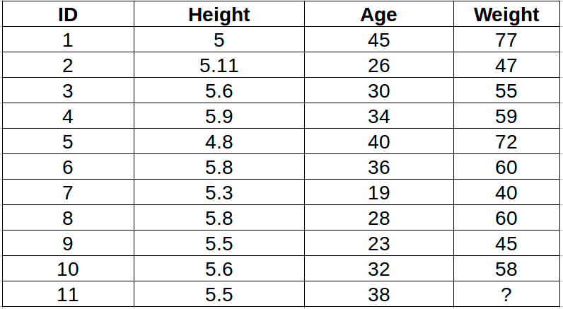
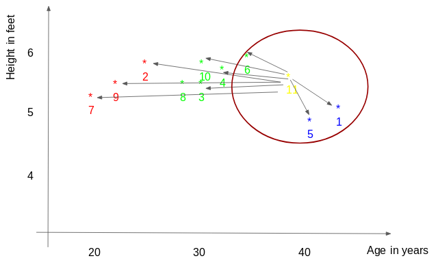
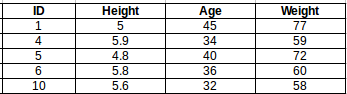
Let us start with a simple example. Consider the following table – it consists of the height, age and weight (target) value for 10 people. As you can see, the weight value of ID11 is missing. We need to predict the weight of this person based on their height and age.

Note: The data in this table does not represent actual values. It is merely used as an example to explain this concept.

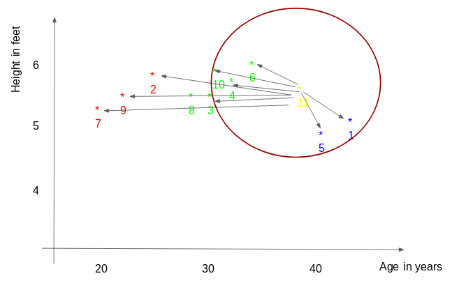
For a clearer understanding of this, below is the plot of height versus age from the above table:

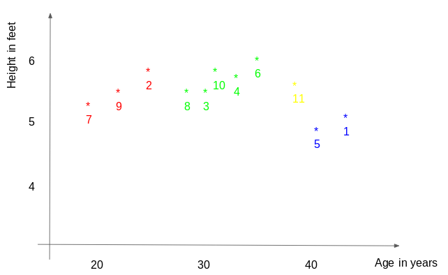
In the above graph, the y-axis represents the height of a person (in feet) and the x-axis represents the age (in years). The points are numbered according to the ID values. The yellow point (ID 11) is our test point.

If I ask you to identify the weight of ID11 based on the plot, what would be your answer? You would likely say that since ID11 is closer to points 5 and 1, so it must have a weight similar to these IDs, probably between 72-77 kgs (weights of ID1 and ID5 from the table). That actually makes sense, but how do you think the algorithm predicts the values? We will find that out in this article.

Here is a free video-based course to help you understand KNN algorithm – K-Nearest Neighbors (KNN) Algorithm in Python and R

2. How does the KNN algorithm work?

As we saw above, KNN algorithm can be used for both classification and regression problems. The KNN algorithm uses ‘feature similarity’ to predict the values of any new data points. This means that the new point is assigned a value based on how closely it resembles the points in the training set. From our example, we know that ID11 has height and age similar to ID1 and ID5, so the weight would also approximately be the same.

Had it been a classification problem, we would have taken the mode as the final prediction. In this case, we have two values of weight – 72 and 77. Any guesses on how the final value will be calculated? The average of the values is taken to be the final prediction.

Below is a stepwise explanation of the algorithm:

1. First, the distance between the new point and each training point is calculated.

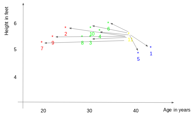
2. The closest k data points are selected (based on the distance). In this example, points 1, 5, 6 will be selected if the value of k is 3. We will further explore the method to select the right value of k later in this article.

 

3. The average of these data points is the final prediction for the new point. Here, we have weight of ID11 = (77+72+60)/3 = 69.66 kg.

In the next few sections, we will discuss each of these three steps in detail.

 

3. Methods of the calculating distance between points

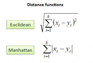
The first step is to calculate the distance between the new point and each training point. There are various methods for calculating this distance, of which the most commonly known methods are – Euclidian, Manhattan (for continuous) and Hamming distance (for categorical).

1. Euclidean Distance: Euclidean distance is calculated as the square root of the sum of the squared differences between a new point (x) and an existing point (y).
2. Manhattan Distance: This is the distance between real vectors using the sum of their absolute difference.
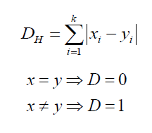
3. Hamming Distance: It is used for categorical variables. If the value (x) and the value (y) are the same, the distance D will be equal to 0 . Otherwise D=1.

Once the distance of a new observation from the points in our training set has been measured, the next step is to pick the closest points. The number of points to be considered is defined by the value of k.

 

4. How to choose the k factor?

The second step is to select the k value. This determines the number of neighbors we look at when we assign a value to any new observation.

In our example, for a value k = 3, the closest points are ID1, ID5 and ID6.

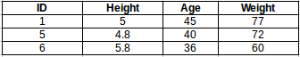
The prediction of weight for ID11 will be:

ID11 = (77+72+60)/3 

ID11 = 69.66 kg

For the value of k=5, the closest point will be ID1, ID4, ID5, ID6, ID10.

The prediction for ID11 will be :

ID 11 =  (77+59+72+60+58)/5 

ID 11 = 65.2 kg

We notice that based on the k value, the final result tends to change. Then how can we figure out the optimum value of k? Let us decide it based on the error calculation for our train and validation set (after all, minimizing the error is our final goal!).

Have a look at the below graphs for training error and validation error for different values of k.

 

For a very low value of k (suppose k=1), the model overfits on the training data, which leads to a high error rate on the validation set. On the other hand, for a high value of k, the model performs poorly on both train and validation set. If you observe closely, the validation error curve reaches a minima at a value of k = 9. This value of k is the optimum value of the model (it will vary for different datasets). This curve is known as an ‘elbow curve‘ (because it has a shape like an elbow) and is usually used to determine the k value.

You can also use the grid search technique to find the best k value. We will implement this in the next section.

 

5. Work on a dataset (Python codes)

By now you must have a clear understanding of the algorithm. If you have any questions regarding the same, please use the comments section below and I will be happy to answer them. We will now go ahead and implement the algorithm on a dataset. I have used the Big Mart sales dataset to show the implementation and you can download it from this link.

The full Python code is below but we have a really cool coding window here where you can code your own k-Nearest Neighbor model in Python:

1. Read the file

import pandas as pd
df = pd.read_csv('train.csv')
df.head()

 

2. Impute missing values

df.isnull().sum()
#missing values in Item_weight and Outlet_size needs to be imputed
mean = df['Item_Weight'].mean() #imputing item_weight with mean
df['Item_Weight'].fillna(mean, inplace =True)

mode = df['Outlet_Size'].mode() #imputing outlet size with mode
df['Outlet_Size'].fillna(mode[0], inplace =True)

 

3. Deal with categorical variables and drop the id columns

df.drop(['Item_Identifier', 'Outlet_Identifier'], axis=1, inplace=True)
df = pd.get_dummies(df)

 

4. Create train and test set

from sklearn.model_selection import train_test_split
train , test = train_test_split(df, test_size = 0.3)

x_train = train.drop('Item_Outlet_Sales', axis=1)
y_train = train['Item_Outlet_Sales']

x_test = test.drop('Item_Outlet_Sales', axis = 1)
y_test = test['Item_Outlet_Sales']

5. Preprocessing – Scaling the features

from sklearn.preprocessing import MinMaxScaler
scaler = MinMaxScaler(feature_range=(0, 1))

x_train_scaled = scaler.fit_transform(x_train)
x_train = pd.DataFrame(x_train_scaled)

x_test_scaled = scaler.fit_transform(x_test)
x_test = pd.DataFrame(x_test_scaled)

 

6. Let us have a look at the error rate for different k values

#import required packages
from sklearn import neighbors
from sklearn.metrics import mean_squared_error 
from math import sqrt
import matplotlib.pyplot as plt
%matplotlib inline

rmse_val = [] #to store rmse values for different k
for K in range(20):
    K = K+1
    model = neighbors.KNeighborsRegressor(n_neighbors = K)

    model.fit(x_train, y_train)  #fit the model
    pred=model.predict(x_test) #make prediction on test set
    error = sqrt(mean_squared_error(y_test,pred)) #calculate rmse
    rmse_val.append(error) #store rmse values
    print('RMSE value for k= ' , K , 'is:', error)

Output :

RMSE value for k = 1 is: 1579.8352322344945
RMSE value for k = 2 is: 1362.7748806138618
RMSE value for k = 3 is: 1278.868577489459
RMSE value for k = 4 is: 1249.338516122638
RMSE value for k = 5 is: 1235.4514224035129
RMSE value for k = 6 is: 1233.2711649472913
RMSE value for k = 7 is: 1219.0633086651026
RMSE value for k = 8 is: 1222.244674933665
RMSE value for k = 9 is: 1219.5895059285074
RMSE value for k = 10 is: 1225.106137547365
RMSE value for k = 11 is: 1229.540283771085
RMSE value for k = 12 is: 1239.1504407152086
RMSE value for k = 13 is: 1242.3726040709887
RMSE value for k = 14 is: 1251.505810196545
RMSE value for k = 15 is: 1253.190119191363
RMSE value for k = 16 is: 1258.802262564038
RMSE value for k = 17 is: 1260.884931441893
RMSE value for k = 18 is: 1265.5133661294733
RMSE value for k = 19 is: 1269.619416217394
RMSE value for k = 20 is: 1272.10881411344

 

#plotting the rmse values against k values
curve = pd.DataFrame(rmse_val) #elbow curve 
curve.plot()

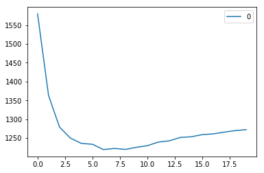
As we discussed, when we take k=1, we get a very high RMSE value. The RMSE value decreases as we increase the k value. At k= 7, the RMSE is approximately 1219.06, and shoots up on further increasing the k value. We can safely say that k=7 will give us the best result in this case.

These are the predictions using our training dataset. Let us now predict the values for test dataset and make a submission.

7. Predictions on the test dataset

#reading test and submission files
test = pd.read_csv('test.csv')
submission = pd.read_csv('SampleSubmission.csv')
submission['Item_Identifier'] = test['Item_Identifier']
submission['Outlet_Identifier'] = test['Outlet_Identifier']

#preprocessing test dataset
test.drop(['Item_Identifier', 'Outlet_Identifier'], axis=1, inplace=True)
test['Item_Weight'].fillna(mean, inplace =True)
test = pd.get_dummies(test)
test_scaled = scaler.fit_transform(test)
test = pd.DataFrame(test_scaled)

#predicting on the test set and creating submission file
predict = model.predict(test)
submission['Item_Outlet_Sales'] = predict
submission.to_csv('submit_file.csv',index=False)

On submitting this file, I get an RMSE of 1279.5159651297.

8. Implementing GridsearchCV 

For deciding the value of k, plotting the elbow curve every time is be a cumbersome and tedious process. You can simply use gridsearch to find the best value.

from sklearn.model_selection import GridSearchCV
params = {'n_neighbors':[2,3,4,5,6,7,8,9]}

knn = neighbors.KNeighborsRegressor()

model = GridSearchCV(knn, params, cv=5)
model.fit(x_train,y_train)
model.best_params_

Output :

{'n_neighbors': 7}

 

6. End Notes and additional resources

In this article, we covered the workings of the KNN algorithm and its implementation in Python. It’s one of the most basic, yet effective machine learning techniques. For KNN implementation in R, you can go through this article : kNN Algorithm using R. You can also go fou our free course – K-Nearest Neighbors (KNN) Algorithm in Python and R to further your foundations of KNN.

In this article, we used the KNN model directly from the sklearn library. You can also implement KNN from scratch (I recommend this!), which is covered in the this article: KNN simplified.

If you think you know KNN well and have a solid grasp on the technique, test your skills in this MCQ quiz: 30 questions on kNN Algorithm. Good luck!