Overview

• Neural Networks are one of the most popular machine learning algorithms
• Gradient Descent forms the basis of Neural networks
• Neural networks can be implemented in both R and Python using certain libraries and packages

Introduction

You can learn and practice a concept in two ways:

• Option 1: You can learn the entire theory on a particular subject and then look for ways to apply those concepts. So, you read up how an entire algorithm works, the maths behind it, its assumptions, limitations and then you apply it. Robust but time taking approach.
• Option 2: Start with simple basics and develop an intuition on the subject. Next, pick a problem and start solving it. Learn the concepts while you are solving the problem. Keep tweaking and improving your understanding. So, you read up how to apply an algorithm – go out and apply it. Once you know how to apply it, try it around with different parameters, values, limits and develop an understanding of the algorithm.

I prefer Option 2 and take that approach to learning any new topic. I might not be able to tell you the entire math behind an algorithm, but I can tell you the intuition. I can tell you the best scenarios to apply an algorithm based on my experiments and understanding.

In my interactions with people, I find that people don’t take time to develop this intuition and hence they struggle to apply things in the right manner.

In this article, I will discuss the building block of a neural network from scratch and focus more on developing this intuition to apply Neural networks. We will code in both “Python” and “R”. By end of this article, you will understand how Neural networks work, how do we initialize weigths and how do we update them using back-propagation.

Let’s start.

 

Table of Contents:

1. Simple intuition behind Neural networks
2. Multi Layer Perceptron and its basics
3. Steps involved in Neural Network methodology
4. Visualizing steps for Neural Network working methodology
5. Implementing NN using Numpy (Python)
6. Implementing NN using R
7. [Optional] Mathematical Perspective of Back Propagation Algorithm

 

Simple intuition behind neural networks

If you have been a developer or seen one work – you know how it is to search for bugs in a code. You would fire various test cases by varying the inputs or circumstances and look for the output. The change in output provides you a hint on where to look for the bug – which module to check, which lines to read. Once you find it, you make the changes and the exercise continues until you have the right code / application.

Neural networks work in very similar manner. It takes several input, processes it through multiple neurons from multiple hidden layers and returns the result using an output layer. This result estimation process is technically known as “Forward Propagation“.

Next, we compare the result with actual output. The task is to make the output to neural network as close to actual (desired) output. Each of these neurons are contributing some error to final output. How do you reduce the error?

We try to minimize the value/ weight of neurons those are contributing more to the error and this happens while traveling back to the neurons of the neural network and finding where the error lies. This process is known as “Backward Propagation“.

In order to reduce these number of iterations to minimize the error, the neural networks use a common algorithm known as “Gradient Descent”, which helps to optimize the task quickly and efficiently.

That’s it – this is how Neural network works! I know this is a very simple representation, but it would help you understand things in a simple manner.

Multi Layer Perceptron and its basics

Just like atoms form the basics of any material on earth – the basic forming unit of a neural network is a perceptron. So, what is a perceptron?

A perceptron can be understood as anything that takes multiple inputs and produces one output. For example, look at the image below.

The above structure takes three inputs and produces one output. The next logical question is what is the relationship between input and output? Let us start with basic ways and build on to find more complex ways.

Below, I have discussed three ways of creating input output relationships:

1. By directly combining the input and computing the output based on a threshold value. for eg: Take x1=0, x2=1, x3=1 and setting a threshold =0. So, if x1+x2+x3>0, the output is 1 otherwise 0. You can see that in this case, the perceptron calculates the output as 1.
2. Next, let us add weights to the inputs. Weights give importance to an input. For example, you assign w1=2, w2=3 and w3=4 to x1, x2 and x3 respectively. To compute the output, we will multiply input with respective weights and compare with threshold value as w1*x1 + w2*x2 + w3*x3 > threshold. These weights assign more importance to x3 in comparison to x1 and x2.
3. Next, let us add bias: Each perceptron also has a bias which can be thought of as how much flexible the perceptron is. It is somehow similar to the constant b of a linear function y = ax + b. It allows us to move the line up and down to fit the prediction with the data better. Without b the line will always goes through the origin (0, 0) and you may get a poorer fit. For example, a perceptron may have two inputs, in that case, it requires three weights. One for each input and one for the bias. Now linear representation of input will look like, w1*x1 + w2*x2 + w3*x3 + 1*b.

But, all of this is still linear which is what perceptrons used to be. But that was not as much fun. So, people thought of evolving a perceptron to what is now called as artificial neuron. A neuron applies non-linear transformations (activation function) to the inputs and biases.

 

What is an activation function?

Activation Function takes the sum of weighted input (w1*x1 + w2*x2 + w3*x3 + 1*b) as an argument and return the output of the neuron. 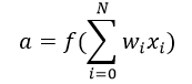In above equation, we have represented 1 as x0 and b as w0.

Forward Propagation, Back Propagation and Epochs

Till now, we have computed the output and this process is known as “Forward Propagation“. But what if the estimated output is far away from the actual output (high error). In the neural network what we do, we update the biases and weights based on the error. This weight and bias updating process is known as “Back Propagation“.

Back-propagation (BP) algorithms work by determining the loss (or error) at the output and then propagating it back into the network. The weights are updated to minimize the error resulting from each neuron. The first step in minimizing the error is to determine the gradient (Derivatives) of each node w.r.t. the final output. To get a mathematical perspective of the Backward propagation, refer below section.

This one round of forward and back propagation iteration is known as one training iteration aka “Epoch“.

Multi-layer perceptron

Now, let’s move on to next part of Multi-Layer Perceptron. So far, we have seen just a single layer consisting of 3 input nodes i.e x1, x2 and x3 and an output layer consisting of a single neuron. But, for practical purposes, the single-layer network can do only so much. An MLP consists of multiple layers called Hidden Layers stacked in between the Input Layer and the Output Layer as shown below.

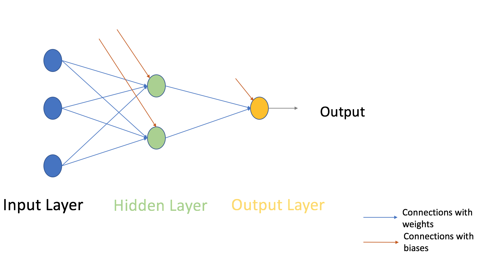
The image above shows just a single hidden layer in green but in practice can contain multiple hidden layers. Another point to remember in case of an MLP is that all the layers are fully connected i.e every node in a layer(except the input and the output layer) is connected to every node in the previous layer and the following layer.

Let’s move on to the next topic which is training algorithm for a neural network (to minimize the error). Here, we will look at most common training algorithm known as Gradient descent.

 

Full Batch Gradient Descent and Stochastic Gradient Descent

Both variants of Gradient Descent perform the same work of updating the weights of the MLP by using the same updating algorithm but the difference lies in the number of training samples used to update the weights and biases.

Full Batch Gradient Descent Algorithm as the name implies uses all the training data points to update each of the weights once whereas Stochastic Gradient uses 1 or more(sample) but never the entire training data to update the weights once.

Let us understand this with a simple example of a dataset of 10 data points with two weights w1 and w2.

Full Batch: You use 10 data points (entire training data) and calculate the change in w1 (Δw1) and change in w2(Δw2) and update w1 and w2.

SGD: You use 1st data point and calculate the change in w1 (Δw1) and change in w2(Δw2) and update w1 and w2. Next, when you use 2nd data point, you will work on the updated weights

For a more in-depth explanation of both the methods, you can have a look at this article.

 

Steps involved in Neural Network methodology

Let’s look at the step by step building methodology of Neural Network (MLP with one hidden layer, similar to above-shown architecture). At the output layer, we have only one neuron as we are solving a binary classification problem (predict 0 or 1). We could also have two neurons for predicting each of both classes.

First look at the broad steps:

0.) We take input and output

• X as an input matrix
• y as an output matrix

1.) We initialize weights and biases with random values (This is one time initiation. In the next iteration, we will use updated weights, and biases). Let us define:

• wh as weight matrix to the hidden layer
• bh as bias matrix to the hidden layer
• wout as weight matrix to the output layer
• bout as bias matrix to the output layer

2.) We take matrix dot product of input and weights assigned to edges between the input and hidden layer then add biases of the hidden layer neurons to respective inputs, this is known as linear transformation:

hidden_layer_input= matrix_dot_product(X,wh) + bh

3) Perform non-linear transformation using an activation function (Sigmoid). Sigmoid will return the output as 1/(1 + exp(-x)).

hiddenlayer_activations = sigmoid(hidden_layer_input)

4.) Perform a linear transformation on hidden layer activation (take matrix dot product with weights and add a bias of the output layer neuron) then apply an activation function (again used sigmoid, but you can use any other activation function depending upon your task) to predict the output

output_layer_input = matrix_dot_product (hiddenlayer_activations * wout ) + bout
output = sigmoid(output_layer_input)

All above steps are known as “Forward Propagation“

5.) Compare prediction with actual output and calculate the gradient of error (Actual – Predicted). Error is the mean square loss = ((Y-t)^2)/2

E = y – output

6.) Compute the slope/ gradient of hidden and output layer neurons ( To compute the slope, we calculate the derivatives of non-linear activations x at each layer for each neuron). Gradient of sigmoid can be returned as x * (1 – x).

slope_output_layer = derivatives_sigmoid(output)
slope_hidden_layer = derivatives_sigmoid(hiddenlayer_activations)

7.) Compute change factor(delta) at output layer, dependent on the gradient of error multiplied by the slope of output layer activation

d_output = E * slope_output_layer

8.) At this step, the error will propagate back into the network which means error at hidden layer. For this, we will take the dot product of output layer delta with weight parameters of edges between the hidden and output layer (wout.T).

Error_at_hidden_layer = matrix_dot_product(d_output, wout.Transpose)

9.) Compute change factor(delta) at hidden layer, multiply the error at hidden layer with slope of hidden layer activation

d_hiddenlayer = Error_at_hidden_layer * slope_hidden_layer

10.) Update weights at the output and hidden layer: The weights in the network can be updated from the errors calculated for training example(s).

wout = wout + matrix_dot_product(hiddenlayer_activations.Transpose, d_output)*learning_rate
wh =  wh + matrix_dot_product(X.Transpose,d_hiddenlayer)*learning_rate

learning_rate: The amount that weights are updated is controlled by a configuration parameter called the learning rate)

11.) Update biases at the output and hidden layer: The biases in the network can be updated from the aggregated errors at that neuron.

• bias at output_layer =bias at output_layer + sum of delta of output_layer at row-wise * learning_rate
• bias at hidden_layer =bias at hidden_layer + sum of delta of output_layer at row-wise * learning_rate   

bh = bh + sum(d_hiddenlayer, axis=0) * learning_rate
bout = bout + sum(d_output, axis=0)*learning_rate

Steps from 5 to 11 are known as “Backward Propagation“

One forward and backward propagation iteration is considered as one training cycle. As I mentioned earlier, When do we train second time then update weights and biases are used for forward propagation.

Above, we have updated the weight and biases for hidden and output layer and we have used full batch gradient descent algorithm.

 

Visualization of steps for Neural Network methodology

We will repeat the above steps and visualize the input, weights, biases, output, error matrix to understand working methodology of Neural Network (MLP).

Note:

• For good visualization images, I have rounded decimal positions at 2 or3 positions.
• Yellow filled cells represent current active cell
• Orange cell represents the input used to populate values of current cell

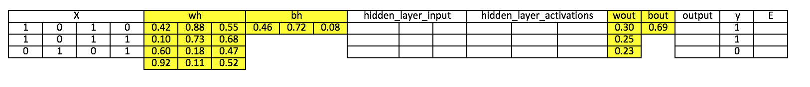
Step 0: Read input and output

Step 1: Initialize weights and biases with random values (There are methods to initialize weights and biases but for now initialize with random values)

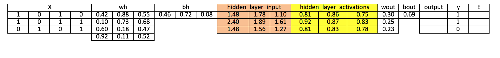
Step 2: Calculate hidden layer input:
hidden_layer_input= matrix_dot_product(X,wh) + bh

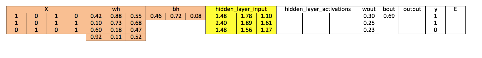Step 3: Perform non-linear transformation on hidden linear input
hiddenlayer_activations = sigmoid(hidden_layer_input)

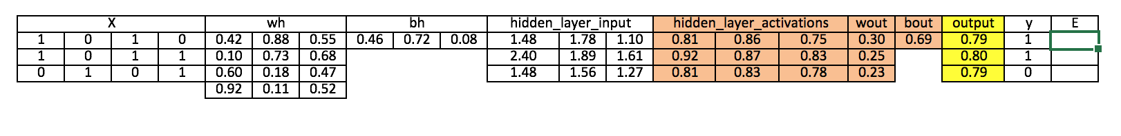
Step 4: Perform linear and non-linear transformation of hidden layer activation at output layer

output_layer_input = matrix_dot_product (hiddenlayer_activations * wout ) + bout
output = sigmoid(output_layer_input)

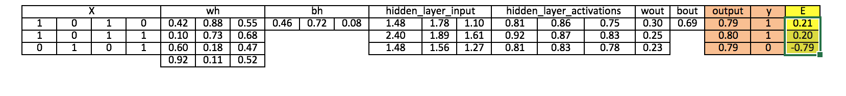
Step 5: Calculate gradient of Error(E) at output layer
E = y-output

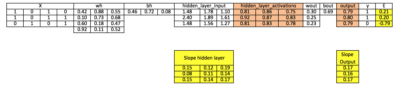
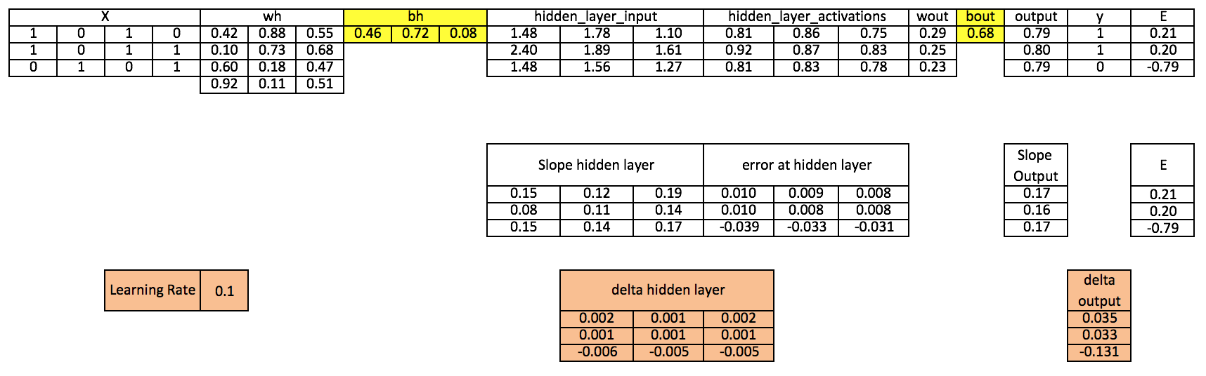
Step 6: Compute slope at output and hidden layer
Slope_output_layer= derivatives_sigmoid(output)
Slope_hidden_layer = derivatives_sigmoid(hiddenlayer_activations)

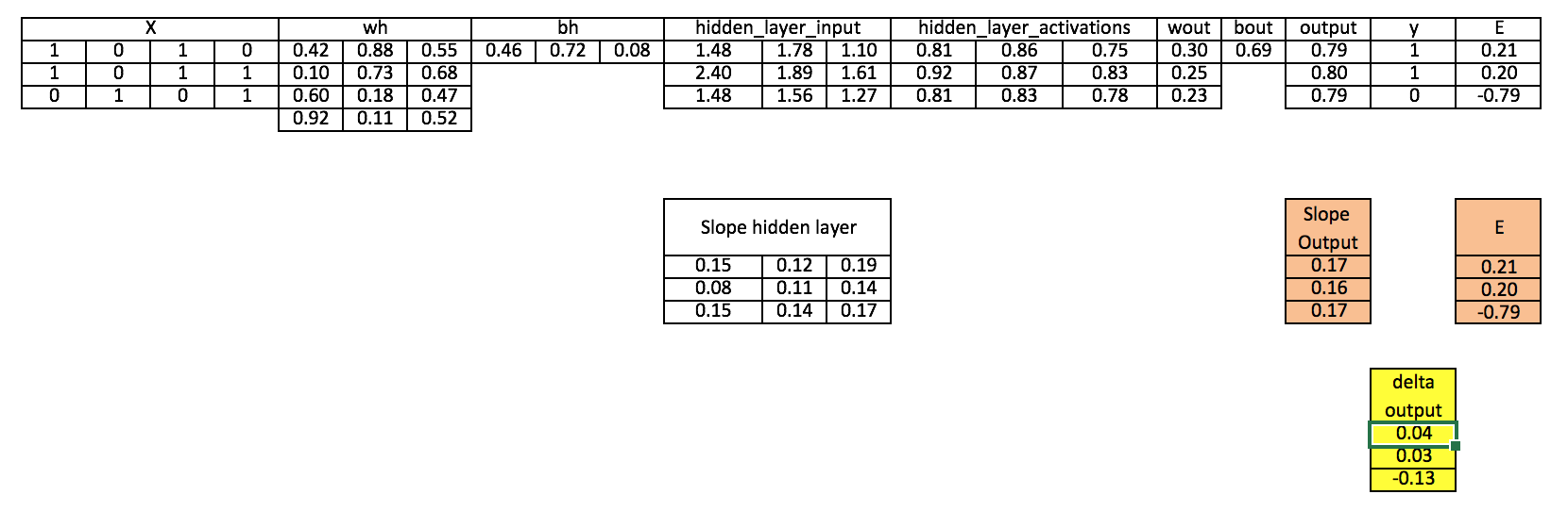
Step 7: Compute delta at output layer

d_output = E * slope_output_layer*lr

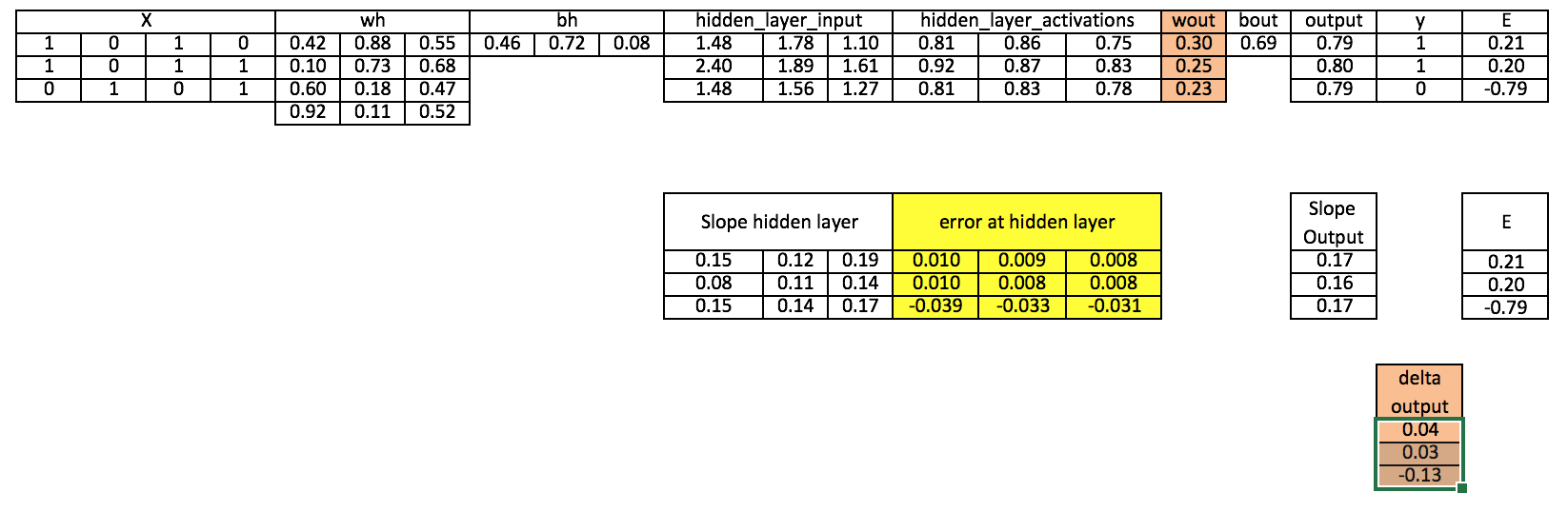
Step 8: Calculate Error at hidden layer

Error_at_hidden_layer = matrix_dot_product(d_output, wout.Transpose)

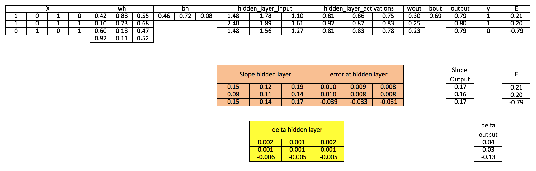
Step 9: Compute delta at hidden layer

d_hiddenlayer = Error_at_hidden_layer * slope_hidden_layer

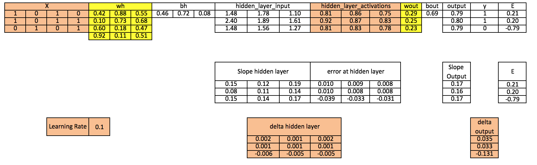
Step 10: Update weight at both output and hidden layer

wout = wout + matrix_dot_product(hiddenlayer_activations.Transpose, d_output)*learning_rate
wh =  wh+ matrix_dot_product(X.Transpose,d_hiddenlayer)*learning_rate

Step 11: Update biases at both output and hidden layer

bh = bh + sum(d_hiddenlayer, axis=0) * learning_rate
bout = bout + sum(d_output, axis=0)*learning_rate

Above, you can see that there is still a good error not close to actual target value because we have completed only one training iteration. If we will train model multiple times then it will be a very close actual outcome. I have completed thousands iteration and my result is close to actual target values ([[ 0.98032096] [ 0.96845624] [ 0.04532167]]).

 

Implementing NN using Numpy (Python)

 

Implementing NN in R

# input matrix
X=matrix(c(1,0,1,0,1,0,1,1,0,1,0,1),nrow = 3, ncol=4,byrow = TRUE)

# output matrix
Y=matrix(c(1,1,0),byrow=FALSE)

#sigmoid function
sigmoid<-function(x){
1/(1+exp(-x))
}

# derivative of sigmoid function
derivatives_sigmoid<-function(x){
x*(1-x)
}

# variable initialization
epoch=5000
lr=0.1
inputlayer_neurons=ncol(X)
hiddenlayer_neurons=3
output_neurons=1

#weight and bias initialization
wh=matrix( rnorm(inputlayer_neurons*hiddenlayer_neurons,mean=0,sd=1), inputlayer_neurons, hiddenlayer_neurons)
bias_in=runif(hiddenlayer_neurons)
bias_in_temp=rep(bias_in, nrow(X))
bh=matrix(bias_in_temp, nrow = nrow(X), byrow = FALSE)
wout=matrix( rnorm(hiddenlayer_neurons*output_neurons,mean=0,sd=1), hiddenlayer_neurons, output_neurons)

bias_out=runif(output_neurons)
bias_out_temp=rep(bias_out,nrow(X))
bout=matrix(bias_out_temp,nrow = nrow(X),byrow = FALSE)
# forward propagation
for(i in 1:epoch){

hidden_layer_input1= X%*%wh
hidden_layer_input=hidden_layer_input1+bh
hidden_layer_activations=sigmoid(hidden_layer_input)
output_layer_input1=hidden_layer_activations%*%wout
output_layer_input=output_layer_input1+bout
output= sigmoid(output_layer_input)

# Back Propagation

E=Y-output
slope_output_layer=derivatives_sigmoid(output)
slope_hidden_layer=derivatives_sigmoid(hidden_layer_activations)
d_output=E*slope_output_layer
Error_at_hidden_layer=d_output%*%t(wout)
d_hiddenlayer=Error_at_hidden_layer*slope_hidden_layer
wout= wout + (t(hidden_layer_activations)%*%d_output)*lr
bout= bout+rowSums(d_output)*lr
wh = wh +(t(X)%*%d_hiddenlayer)*lr
bh = bh + rowSums(d_hiddenlayer)*lr

}
output

 

[Optional] Mathematical Perspective of Back Propagation Algorithm

Let W_i be the weights between the input layer and the hidden layer. W_h be the weights between the hidden layer and the output layer.

Now, h=σ (u)= σ (W_iX), i.e h is a function of u and u is a function of W_i and X. here we represent our function as σ

Y= σ (u’)= σ (W_hh), i.e Y is a function of u’ and u’ is a function of W_h and h.

We will be constantly referencing the above equations to calculate partial derivatives.

We are primarily interested in finding two terms, ∂E/∂W_i and ∂E/∂W_h i.e change in Error on changing the weights between the input and the hidden layer and change in error on changing the weights between the hidden layer and the output layer.

But to calculate both these partial derivatives, we will need to use the chain rule of partial differentiation since E is a function of Y and Y is a function of u’ and u’ is a function of W_i.

Let’s put this property to good use and calculate the gradients.

∂E/∂W_h = (∂E/∂Y).( ∂Y/∂u’).( ∂u’/∂W_h), ……..(1)

We know E is of the form E=(Y-t)²/2.

So, (∂E/∂Y)= (Y-t)

Now, σ is a sigmoid function and has an interesting differentiation of the form σ(1- σ). I urge the readers to work this out on their side for verification.

So, (∂Y/∂u’)= ∂( σ(u’)/ ∂u’= σ(u’)(1- σ(u’)).

But, σ(u’)=Y, So,

(∂Y/∂u’)=Y(1-Y)

Now, ( ∂u’/∂W_h)= ∂( W_hh)/ ∂W_h = h

Replacing the values in equation (1) we get,

∂E/∂W_h = (Y-t). Y(1-Y).h

So, now we have computed the gradient between the hidden layer and the ouput layer. It is time we calculate the gradient between the input layer and the hidden layer.

∂E/∂W_i =(∂ E/∂ h). (∂h/∂u).( ∂u/∂W_i)

But, (∂ E/∂ h) = (∂E/∂Y).( ∂Y/∂u’).( ∂u’/∂h). Replacing this value in the above equation we get,

∂E/∂W_i =[(∂E/∂Y).( ∂Y/∂u’).( ∂u’/∂h)]. (∂h/∂u).( ∂u/∂W_i)……………(2)

So, What was the benefit of first calculating the gradient between the hidden layer and the output layer?

As you can see in equation (2) we have already computed ∂E/∂Y and ∂Y/∂u’ saving us space and computation time. We will come to know in a while why is this algorithm called the back propagation algorithm.

Let us compute the unknown derivatives in equation (2).

∂u’/∂h = ∂(W_hh)/ ∂h = W_h

∂h/∂u = ∂( σ(u)/ ∂u= σ(u)(1- σ(u))

But, σ(u)=h, So,

(∂Y/∂u)=h(1-h)

Now, ∂u/∂W_i = ∂(W_iX)/ ∂W_i = X

Replacing all these values in equation (2) we get,

∂E/∂W_i = [(Y-t). Y(1-Y).W_h].h(1-h).X

So, now since we have calculated both the gradients, the weights can be updated as

W_h = W_h + η . ∂E/∂W_h

W_i = W_i + η . ∂E/∂W_i

Where η is the learning rate.

So coming back to the question: Why is this algorithm called Back Propagation Algorithm?

The reason is: If you notice the final form of ∂E/∂W_h and ∂E/∂W_i , you will see the term (Y-t) i.e the output error, which is what we started with and then propagated this back to the input layer for weight updation.

So, where does this mathematics fit into the code?

hiddenlayer_activations=h

E= Y-t

Slope_output_layer = Y(1-Y)

lr = η

slope_hidden_layer = h(1-h)

wout = W_h

Now, you can easily relate the code to the mathematics.

 

End Notes:

This article is focused on the building a Neural Network from scratch and understanding its basic concepts. I hope now you understand the working of a neural network like how does forward and backward propagation work, optimization algorithms (Full Batch and Stochastic gradient descent),  how to update weights and biases, visualization of each step in Excel and on top of that code in python and R.

Therefore, in my upcoming article, I’ll explain the applications of using Neural Network in Python and solving real-life challenges related to:

1. Computer Vision
2. Speech
3. Natural Language Processing

I enjoyed writing this article and would love to learn from your feedback. Did you find this article useful? I would appreciate your suggestions/feedback. Please feel free to ask your questions through comments below.

Learn, compete, hack and get hired!