Learn How to Use Support Vector Machines (SVM) for Data Science

Mastering machine learning algorithms isn’t a myth at all. Most beginners start by learning regression. It is simple to learn and use, but does that solve our purpose? Of course not! Because there is a lot more in ML beyond logistic regression and regression problems! For instance, have you heard of support vector regression and support vector machines or SVM?

Think of machine learning algorithms as an armory packed with axes, swords, blades, bows, daggers, etc. You have various tools, but you ought to learn to use them at the right time. As an analogy, think of ‘Regression’ as a sword capable of slicing and dicing data efficiently but incapable of dealing with highly complex data. That is where ‘Support Vector Machines’ acts like a sharp knife – it works on smaller datasets, but on complex ones, it can be much stronger and more powerful in building machine learning models.

Learning Objectives

• Understand support vector machine algorithm (SVM), a popular machine learning algorithm or classification.
• Learn to implement SVM models in R and Python.
• Know the pros and cons of Support Vector Machines (SVM) and their different applications in machine learning (artificial intelligence).

Helpful Resources

By now, I hope you’ve now mastered Random Forest, Naive Bayes Algorithm, and Ensemble Modeling. If not, I’d suggest you take a few minutes and read about them. In this article, I shall guide you through the basics to advanced knowledge of a crucial machine learning algorithm, support vector machines.

You can learn about Support Vector Machines in course format with this tutorial (it’s free!) – SVM in Python and R

If you’re a beginner looking to start your data science journey, you’ve come to the right place! Check out the below comprehensive courses, curated by industry experts, that we have created just for you:

• Introduction to Data Science
• Machine Learning Certification Course for Beginners
• Certified AI & ML Blackbelt+ Program

What Is a Support Vector Machine (SVM)?

“Support Vector Machine” (SVM) is a supervised learning machine learning algorithm that can be used for both classification or regression challenges. However, it is mostly used in classification problems, such as text classification. In the SVM algorithm, we plot each data item as a point in n-dimensional space (where n is the number of features you have), with the value of each feature being the value of a particular coordinate. Then, we perform classification by finding the optimal hyper-plane that differentiates the two classes very well (look at the below snapshot).

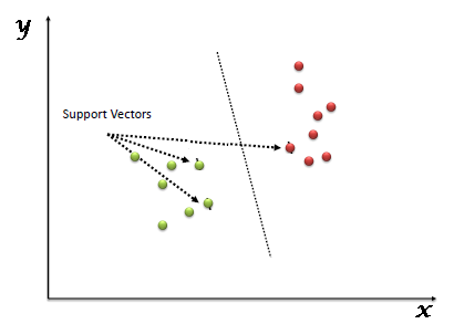
Support Vectors are simply the coordinates of individual observation, and a hyper-plane is a form of SVM visualization. The SVM classifier is a frontier that best segregates the two classes (hyper-plane/line).

How Does a Support Vector Machine / SVM Work?

Above, we got accustomed to the process of segregating the two classes with a hyper-plane. Now the burning question is, “How can we identify the right hyper-plane?”. Don’t worry; it’s not as hard as you think! Let’s understand:

Identify the Right Hyper-plane

• Here, we have three hyper-planes (A, B, and C). Now, identify the right hyper-plane to classify stars and circles.
• You need to remember a thumb rule to identify the right hyper-plane: “Select the hyper-plane which segregates the two classes better.” In this scenario, hyper-plane “B” has excellently performed this job.

Another Example of Identifying the Right Hyper-plane

• Here, we have three hyper-planes (A, B, and C), and all segregate the classes well. Now, How can we identify the right hyper-plane?

• Here, maximizing the distances between the nearest data point (either class) and the hyper-plane will help us to decide the right hyper-plane. This distance is called a Margin. Let’s look at the below snapshot:

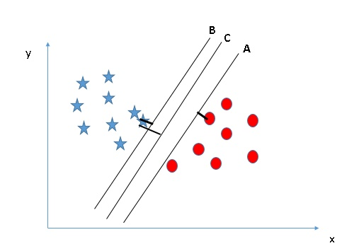
• Above, you can see that the margin for hyper-plane C is high as compared to both A and B. Hence, we name the right hyper-plane as C. Another lightning reason for selecting the hyper-plane with a higher margin is robustness. If we select a hyper-plane having a low margin, then there is a high chance of misclassification.

Another Example of Identifing the right hyper-plane

• Hint: Use the rules as discussed in the previous section to identify the right hyper-plane.

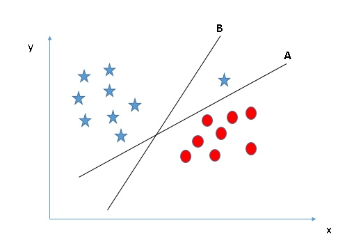
• Some of you may have selected hyper-plane B as it has a higher margin compared to A. But, here is the catch, SVM selects the hyper-plane which classifies the classes accurately prior to maximizing the margin. Here, hyper-plane B has a classification error, and A has classified all correctly. Therefore, the right hyper-plane is A.

Can we classify two classes 

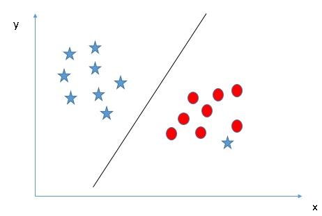
• Below, I am unable to segregate the two classes using a straight line, as one of the stars lies in the territory of the other (circle) class as an outlier.

• As I have already mentioned, one star at the other end is like an outlier for the star class. The SVM algorithm has a feature to ignore outliers and find the hyper-plane that has the maximum margin. Hence, we can say SVM classification is robust to outliers.

Find the Hyper-plane to Segregate to Classes

• In the scenario below, we can’t have a linear hyper-plane between the two classes, so how does SVM classify these two classes? Till now, we have only looked at the linear hyper-plane.

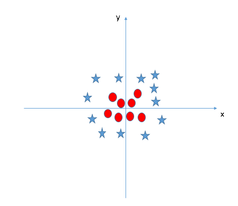
• SVM can solve this problem. Easily! It solves this problem by introducing additional features. Here, we will add a new feature, z=x^2+y^2. Now, let’s plot the data points on axis x and z:

In the above plot, points to consider are:

• All values for z would always be positive because z is the squared sum of both x and y
• In the original plot, red circles appear close to the origin of the x and y axes, leading to a lower value of z. The star is relatively away from the original results due to the higher value of z.

In the SVM classifier, having a linear hyper-plane between these two classes is easy. But, another burning question that arises is if we should we need to add this feature manually to have a hyper-plane. No, the SVM  algorithm has a technique called the kernel trick. The SVM kernel is a function that takes low dimensional input space and transforms it to a higher dimensional space, i.e., it converts not separable problem to a separable problem. It is mostly useful in non-linear data separation problems. Simply put, it does some extremely complex data transformations, then finds out the process to separate the data based on the labels or outputs you’ve defined.

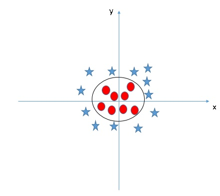
When we look at the hyper-plane in the original input space, it looks like a circle:

Now, let’s look at the methods to apply the SVM classifier algorithm in a data science challenge.

You can also learn about the working of a Support Vector Machine in video format from this Machine Learning certification course.

How to Implement SVM in Python and R?

In Python, scikit-learn is a widely used library for implementing machine learning algorithms. SVM is also available in the scikit-learn library, and we follow the same structure for using it(Import library, object creation, fitting model, and prediction).

Now, let us have a look at a real-life problem statement and dataset to understand how to apply SVM for classification.

Problem Statement

Dream Housing Finance company deals in all home loans. They have a presence across all urban, semi-urban, and rural areas. A customer first applies for a home loan; after that, the company validates the customer’s eligibility for a loan.

The company wants to automate the loan eligibility process (real-time) based on customer details provided while filling out an online application form. These details are Gender, Marital Status, Education, Number of Dependents, Income, Loan Amount, Credit History, and others. To automate this process, they have given a problem of identifying the customers’ segments that are eligible for loan amounts so that they can specifically target these customers. Here they have provided a partial data set.

Use the coding window below to predict the loan eligibility on the test set(new data). Try changing the hyperparameters for the linear SVM to improve the accuracy.

Support Vector Machine (SVM) Code in R

The e1071 package in R is used to create Support Vector Machines with ease. It has helper functions as well as code for the Naive Bayes Classifier. The creation of a support vector machine in R and Python follows similar approaches; let’s take a look now at the following code:

#Import Library
require(e1071) #Contains the SVM 
Train <- read.csv(file.choose())
Test <- read.csv(file.choose())
# there are various options associated with SVM training; like changing kernel, gamma and C value.

# create model
model <- svm(Target~Predictor1+Predictor2+Predictor3,data=Train,kernel='linear',gamma=0.2,cost=100)

#Predict Output
preds <- predict(model,Test)
table(preds)

How to Tune the Parameters of SVM?

Tuning the parameters’ values for machine learning algorithms effectively improves model performance. Let’s look at the list of parameters available with SVM.

sklearn.svm.SVC(C=1.0, kernel='rbf', degree=3, gamma=0.0, coef0=0.0, shrinking=True, probability=False,tol=0.001, cache_size=200, class_weight=None, verbose=False, max_iter=-1, random_state=None)

I am going to discuss some important parameters having a higher impact on model performance, “kernel,” “gamma,” and “C.”

kernel: We have already discussed it. Here, we have various options available with kernel like “linear,” “rbf”, ”poly”, and others (default value is “rbf”).  Here “rbf”(radial basis function) and “poly”(polynomial kernel) are useful for non-linear hyper-plane. It’s called nonlinear svm. Let’s look at the example where we’ve used linear kernel on two features of the iris data set to classify their class.

Support Vector Machine (SVM) Code in Python

Example: Have a linear SVM kernel

import numpy as np
import matplotlib.pyplot as plt
from sklearn import svm, datasets

# import some data to play with
iris = datasets.load_iris()
X = iris.data[:, :2] # we only take the first two features. We could
 # avoid this ugly slicing by using a two-dim dataset
y = iris.target

# we create an instance of SVM and fit out data. We do not scale our
# data since we want to plot the support vectors
C = 1.0 # SVM regularization parameter
svc = svm.SVC(kernel='linear', C=1,gamma=0).fit(X, y)

# create a mesh to plot in
x_min, x_max = X[:, 0].min() - 1, X[:, 0].max() + 1
y_min, y_max = X[:, 1].min() - 1, X[:, 1].max() + 1
h = (x_max / x_min)/100
xx, yy = np.meshgrid(np.arange(x_min, x_max, h),
 np.arange(y_min, y_max, h))

plt.subplot(1, 1, 1)
Z = svc.predict(np.c_[xx.ravel(), yy.ravel()])
Z = Z.reshape(xx.shape)
plt.contourf(xx, yy, Z, cmap=plt.cm.Paired, alpha=0.8)

Example: Use SVM rbf kernel

plt.scatter(X[:, 0], X[:, 1], c=y, cmap=plt.cm.Paired)
plt.xlabel('Sepal length')
plt.ylabel('Sepal width')
plt.xlim(xx.min(), xx.max())
plt.title('SVC with linear kernel')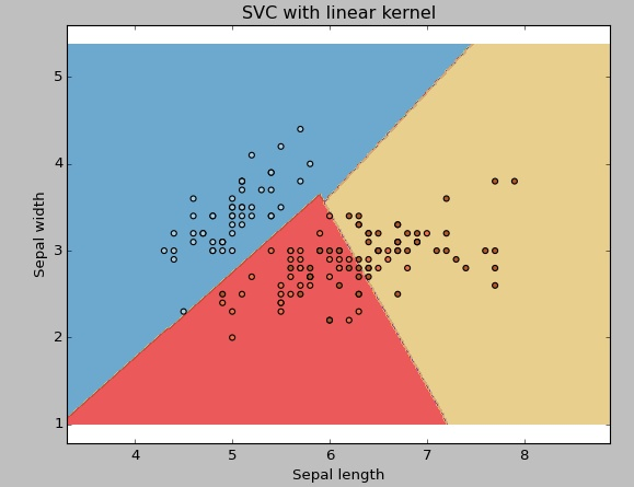

plt.show()

Example: Use SVM rbf kernel

Change the kernel function type to rbf in the below line and look at the impact.

svc = svm.SVC(kernel='rbf', C=1,gamma=0).fit(X, y)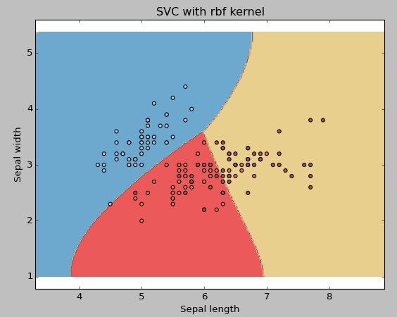

I would suggest you go for a linear SVM kernel if you have a large number of features (>1000) because it is more likely that the data is linearly separable in high dimensional space. Also, you can use RBF but do not forget to cross-validate for its parameters to avoid over-fitting.

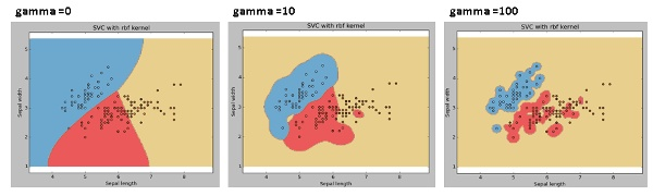
gamma: Kernel coefficient for ‘rbf’, ‘poly’, and ‘sigmoid.’ The higher value of gamma will try to fit them exactly as per the training data set, i.e., generalization error and cause over-fitting problem.

Example: Let’s differentiate if we have gamma different gamma values like 0, 10, or 100.

svc = svm.SVC(kernel=’rbf’, C=1,gamma=0).fit(X, y)

C: Penalty parameter C of the error term. It also controls the trade-off between smooth decision boundaries and classifying the training points correctly.

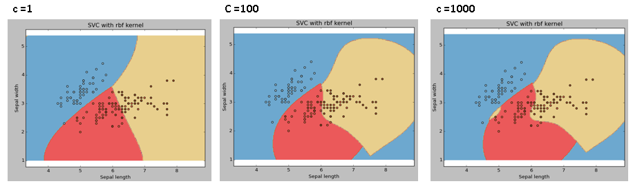
We should always look at the cross-validation score to effectively combine these parameters and avoid over-fitting.

In R, SVMs can be tuned in a similar fashion as they are in Python. Mentioned below are the respective parameters for the e1071 package:

• The kernel parameter can be tuned to take “Linear”, ”Poly”, ”rbf”, etc.
• The gamma value can be tuned by setting the “Gamma” parameter.
• The C value in Python is tuned by the “Cost” parameter in R.

Pros and Cons of SVM

Pros:

• It works really well with a clear margin of separation.
• It is effective in high-dimensional spaces.
• It is effective in cases where the number of dimensions is greater than the number of samples.
• It uses a subset of the training set in the decision function (called support vectors), so it is also memory efficient.

Cons:

• It doesn’t perform well when we have a large data set because the required training time is higher.
• It also doesn’t perform very well when the data set has more noise, i.e., target classes are overlapping.
• SVM doesn’t directly provide probability estimates; these are calculated using an expensive five-fold cross-validation. It is included in the related SVC method of the Python scikit-learn library.

SVM Practice Problem

Find the right additional feature to have a hyper-plane for segregating the classes in the below snapshot:

Answer the variable name in the comments section below. I’ll then reveal the answer.

Conclusion

In this article, we looked at the machine learning algorithm, Support Vector Machine, in detail. We discussed the concept of its working, the process of its implementation in python and R, and the tricks to make the model more efficient by tuning its parameters. Towards the end, we also pointed out the pros and cons of the algorithm. I suggest you try solving the problem above to practice your SVM skills and also try to analyze the power of this model by tuning the parameters.

Key Takeaways

• Support Vector Machines is a strong and powerful algorithm that is best used to build machine learning models with small data sets.
• You can effectively improve your model’s performance by tuning the SVM hyperparameters in Python.
• The algorithm works best when the number of dimensions is greater than the number of samples and is not recommended to be used for noisy, large, or complex data sets.

Frequently Asked Questions

sunil