Framework and Applications of ARIMA time series models

Quick Recap

Hopefully, you would have gained useful insights on time series concepts by now. If not, don’t worry! You can quickly glance through the series of time series articles: Step by Step guide to Learn Time Series, Time Series in R, ARMA Time Series Model. This is the fourth & final article of this series.

A quick revision, till this point we have covered various concepts of ARIMA modelling in bits and pieces. Now is the time to join these pieces and make an interesting story.

In this article we will take you through a comprehensive framework to build a time series model.  In addition, we’ll also discuss about the practical applications of time series modelling.

Overview of the Framework

This framework(shown below) specifies the step by step approach on ‘How to do a Time Series Analysis’:

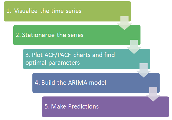
As you would be aware, the first three steps have already been discussed in detail in previous articles. Nevertheless, the same has been delineated briefly below:

Step 1: Visualize the time series

It is very essential to analyze the trends prior to building any kind of time series model. The details we are interested in pertains to any kind of trend, seasonality or random behaviour in the series. We have covered this part in the second part of this series.

Step 2: Stationarize the series

Once we know the patterns, trends, cycles and seasonality , we can check if the series is stationary or not. Dickey – Fuller is one of the popular test to check the same. We have covered this test in the first part of this article series. This doesn’t ends here! What if the series is found to be non-stationary?

There are three commonly used technique to make a time series stationary:

1.  Detrending : Here, we simply remove the trend component from the time series. For instance, the equation of my time series is:

x(t) = (mean + trend * t) + error

We’ll simply remove the part in the parentheses and build model for the rest.

2. Differencing : This is the commonly used technique to remove non-stationarity. Here we try to model the differences of the terms and not the actual term. For instance,

x(t) – x(t-1) = ARMA (p ,  q)

This differencing is called as the Integration part in AR(I)MA. Now, we have three parameters

p : AR

d : I

q : MA

3. Seasonality : Seasonality can easily be incorporated in the ARIMA model directly. More on this has been discussed in the applications part below.

Step 3: Find optimal parameters

The parameters p,d,q can be found using  ACF and PACF plots. An addition to this approach is can be, if both ACF and PACF decreases gradually, it indicates that we need to make the time series stationary and introduce a value to “d”.

Step 4: Build ARIMA model

With the parameters in hand, we can now try to build ARIMA model. The value found in the previous section might be an approximate estimate and we need to explore more (p,d,q) combinations. The one with the lowest BIC and AIC should be our choice. We can also try some models with a seasonal component. Just in case, we notice any seasonality in ACF/PACF plots.

Step 5: Make Predictions

Once we have the final ARIMA model, we are now ready to make predictions on the future time points. We can also visualize the trends to cross validate if the model works fine.

Applications of Time Series Model

In this part, we’ll use the same example that we had used in the previous article. Then, using time series, we’ll make future predictions. We recommend you to check out the example before proceeding further.

Where did we start ?

Following is the plot of the number of passengers with years. Try and make observations on this plot before moving further in the article.

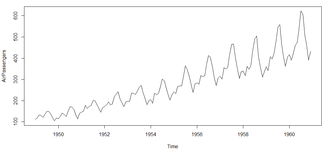
Here are my observations :

1. There is a trend component which grows the passenger year by year.

2. There looks to be a seasonal component which has a cycle less than 12 months.

3. The variance in the data keeps on increasing with time.

Let’s get started

We know that we need to address two issues before we test stationary series. One, we need to remove unequal variances. We do this using log of the series. Two, we need to address the trend component. We do this by taking difference of the series. Now, let’s test the resultant series.

adf.test(diff(log(AirPassengers)), alternative="stationary", k=0)

Augmented Dickey-Fuller Test

data: diff(log(AirPassengers))
 Dickey-Fuller = -9.6003, Lag order = 0,
 p-value = 0.01
 alternative hypothesis: stationary

We see that the series is stationary enough to do any kind of time series modelling.

Next step is to find the right parameters to be used in the ARIMA model. We already know that the ‘d’ component is 1 as we need 1 difference to make the series stationary. We do this using the Correlation plots. Following are the ACF plots for the series :

ACF Plots

acf(log(AirPassengers))

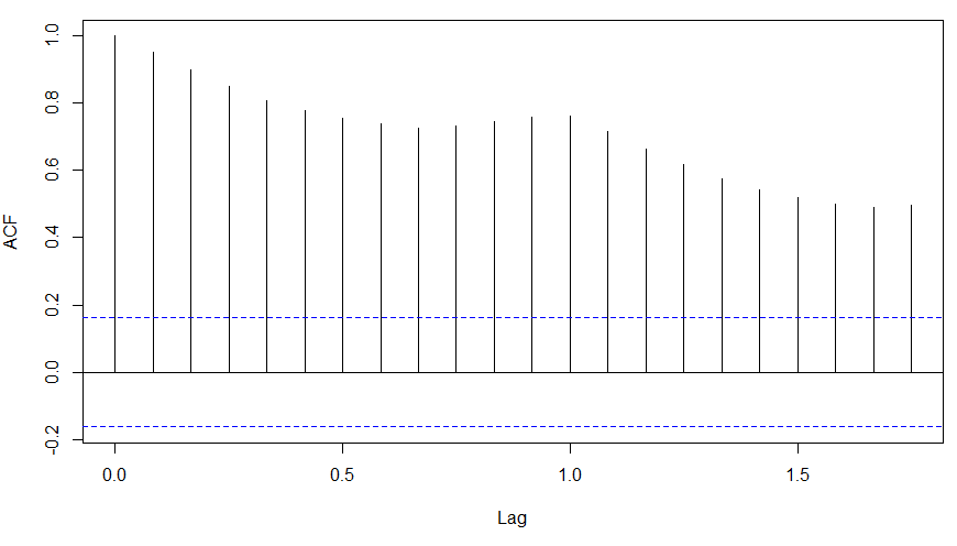
What do you see in the above chart?

Clearly, the decay of ACF chart is very slow, which means that the population is not stationary. We have already discussed above that we now intend to regress on the difference of logs rather than log directly. Let’s see how ACF and PACF curve come out after regressing on the difference.

acf(diff(log(AirPassengers)))

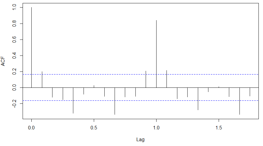
pacf(diff(log(AirPassengers)))

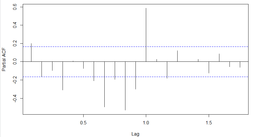
Clearly, ACF plot cuts off after the first lag. Hence, we understood that value of p should be 0 as the ACF is the curve getting a cut off. While value of q should be 1 or 2. After a few iterations, we found that (0,1,1) as (p,d,q) comes out to be the combination with least AIC and BIC.

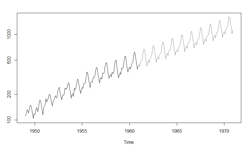
Let’s fit an ARIMA model and predict the future 10 years. Also, we will try fitting in a seasonal component in the ARIMA formulation. Then, we will visualize the prediction along with the training data. You can use the following code to do the same :

(fit <- arima(log(AirPassengers), c(0, 1, 1),seasonal = list(order = c(0, 1, 1), period = 12)))

pred <- predict(fit, n.ahead = 10*12)

ts.plot(AirPassengers,2.718^pred$pred, log = "y", lty = c(1,3))

End Notes

With this article, we have completed the tutorial on ARIMA. Furthermore, the predictions appear to be seamless when we look along with the training data. We are also able to bring out increasing variance, trend, seasonality in the prediction.

The tools mentioned in this article will help you fit in a time series model wherever possible. In a nutshell:

• We visualized the series
• Next, we took a difference to make the trend stationary.
• We then made a Log transformation to account for the increasing variance,
• Brought a seasonal component in ARIMA model to account for annual seasonality; and
• Found the right values for the (p,d,q) combination.

Did you find the article useful? Share with us if you have done similar kind of analysis before. Do let us know your thoughts about this article in the box below.

If you like what you just read & want to continue your analytics learning, subscribe to our emails, follow us on twitter or like our facebook page.

Tavish