Introduction to ARMA Time Series Models – Simplified

ARMA models are commonly used for time series modeling. In ARMA model, AR stands for auto-regression and MA stands for moving average. If the sound of these words is scaring you, worry not – we will simplify these concepts in next few minutes for you!

Pedagogy

In this article, we will develop a knack for these terms and understand the characteristics associated with these models. But before we start, you should remember, AR or MA are not applicable on non-stationary series. In case you get a non stationary series, you first need to stationarize the series (by taking difference / transformation) and then choose from the available time series models.

We’ll first begin with explaining each of these two models (AR & MA) individually. Next, we will look at the characteristics of these models. Further, in the coming articles we will focus on how to make an appropriate choice of the right parameters for an ARMA / ARIMA models.

Auto-Regressive Time Series model

Let’s develop an understanding of AR models using the case below:

The current GDP of a country say x(t) is dependent on the last year’s GDP i.e. x(t – 1). The hypothesis being that the total cost of production of products & services in a country in a fiscal year (known as GDP) is dependent on the set up of manufacturing plants / services in the previous year and the newly set up industries / plants / services in the current year. But the primary component of the GDP is the former one.

Hence, we can formally write the equation of GDP as:

x(t) = alpha *  x(t – 1) + error (t)

This equation is known as AR(1) formulation. The numeral one (1) denotes that the next instance is solely dependent on the previous instance.  The alpha is a coefficient which we seek so as to minimize the error function. Notice that x(t- 1) is indeed linked to x(t-2) in the same fashion. Hence, any shock to x(t) will gradually fade off in future.

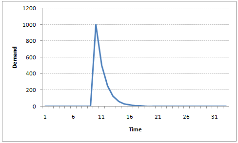
For instance, let’s say x(t) is the number of juice bottles sold in a city on a particular day. During winters, very few vendors purchased juice bottles. Suddenly, on a particular day, the temperature rose and the demand of juice bottles soared to 1000. However, after a few days, the climate became cold again. But, knowing that the people got used to drinking juice during the hot days, there were 50% of the people still drinking juice during the cold days. In following days, the proportion went down to 25% (50% of 50%) and then gradually to a small number after significant number of days. The following graph explains the inertia property of AR series:

Moving Average Time Series Model

Let’s take another case to understand Moving average time series model.

A manufacturer produces a certain type of bag, which was readily available in the market. Being a competitive market, the sale of the bag stood at zero for many days. So, one day he did some experiment with the design and produced a different type of bag. This type of bag was not available anywhere in the market. Thus, he was able to sell the entire stock of 1000 bags (lets call this as x(t) ). The demand got so high that the bag ran out of stock. As a result, some 100 odd customers couldn’t purchase this bag. Lets call this gap as the error at that time point. With time, the bag had lost its woo factor. But still few customers were left who went empty handed the previous day. Following is a simple formulation to depict the scenario :

x(t) = beta *  error(t-1) + error (t)

If we try plotting this graph, it will look something like this :

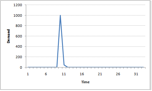
Did you notice the difference between MA and AR model? In MA model, noise / shock quickly vanishes with time. The AR model has a much lasting effect of the shock.

Difference between AR and MA models

The primary difference between an AR and MA model is based on the correlation between time series objects at different time points. The correlation between x(t) and x(t-n) for n > order of MA is always zero. This directly flows from the fact that covariance between x(t) and x(t-n) is zero for MA models (something which we refer from the example taken in the previous section). However, the correlation of x(t) and x(t-n) gradually declines with n becoming larger in the AR model. This difference gets exploited irrespective of having the AR model or MA model. The correlation plot can give us the order of MA model.

Exploiting ACF and PACF plots

Once we have got the stationary time series, we need to answer two primary question:

Q1. Is it an AR or MA process?

Q2. What order of AR or MA process do we need to use?

The trick to solve answer these questions is there in the previous section. Didn’t you notice?

The first question can be answered using Total Correlation Chart (also known as Auto – correlation Function / ACF).  ACF is a plot of total correlation between different lag functions. For instance, in GDP problem, the GDP at time point t is x(t). We are interested in the correlation of x(t) with x(t-1) , x(t-2) and so on. Now let’s reflect on what we have learnt from the previous article. In a moving average series of lag n, we will not get any correlation between x(t) and x(t – n -1) . Hence, the total correlation chart cuts off at nth lag. So it becomes simple to find the lag for a MA series. For an AR series this correlation will gradually go down without any cut off value. So what do we do if it is an AR series?

Here is the second trick. If we find out the partial correlation of each lag, it will cut off after the degree of AR series.  For instance,if we have a AR(1) series,  if we exclude the effect of 1st lag (x (t-1) ), our 2nd lag (x (t-2) ) is independent of x(t). Hence, the partial correlation function (PACF) will drop sharply after the 1st lag. Following are the examples which will clarify any doubts you have on this concept :

                            ACF                                                                      PACF

The blue line above shows significantly different values than zero. Clearly, the graph above has a cut off on PACF curve after 2nd lag which means this is mostly an AR(2) process.

                                      ACF                                                                 PACF

Clearly, the graph above has a cut off on ACF curve after 2nd lag which means this is mostly a MA(2) process.

End Notes

In this article, we have covered on how to identify the type of stationary series using ACF & PACF plots. In the following articles we will discuss on how to stabilize a series and a practical application of time series modelling.

Did you find the article useful? Share with us if you have done similar kind of analysis before. Do let us know your thoughts about this article in the box below.

If you like what you just read & want to continue your analytics learning, subscribe to our emails, follow us on twitter or like our facebook page.

Tavish