Exploration of Time Series Data in R

This is the second part of the step by step guide to Time Series Modelling. In the first part, we looked at basics of time series, stationary series, random walk and Dicky Fuller test. If you have not read this article, I would suggest to go through that first.

In this article we will talk about handling time series data on R. Our scope of this article will be restricted to data exploring in a time series type of dataset and not go to building time series models.  In this article I have used an inbuilt dataset of R called AirPassengers. The dataset consists of monthly totals of international airline passengers, 1949 to 1960. This article will help you explore the data step by step and we will make predictions based on this data for the number of passengers post 1960 in next few articles.

Loading the dataset

Following is the code which will help you load the dataset and spill out a few top level metrics.

> data(AirPassengers)
 > class(AirPassengers)
 [1] "ts"

#This tells you that the data series is in a time series format
 > start(AirPassengers)
 [1] 1949 1

#This is the start of the time series

> end(AirPassengers)
 [1] 1960 12

#This is the end of the time series

> frequency(AirPassengers)
 [1] 12

#The cycle of this time series is 12months in a year
 > summary(AirPassengers)
 Min. 1st Qu. Median Mean 3rd Qu. Max.
 104.0 180.0 265.5 280.3 360.5 622.0

Detailed Metrics

#The number of passengers are distributed across the spectrum

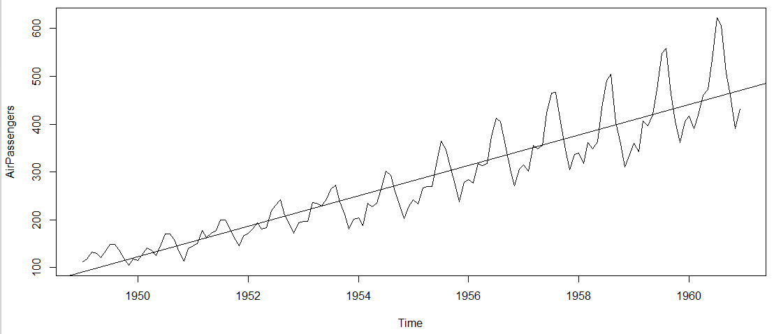
> plot(AirPassengers)

#This will plot the time series

>abline(reg=lm(AirPassengers~time(AirPassengers)))

# This will fit in a line

Here are a few more operations you can do:

> cycle(AirPassengers)

#This will print the cycle across years.

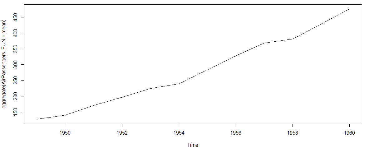
>plot(aggregate(AirPassengers,FUN=mean))

#This will aggreage the cycles and display a year on year trend

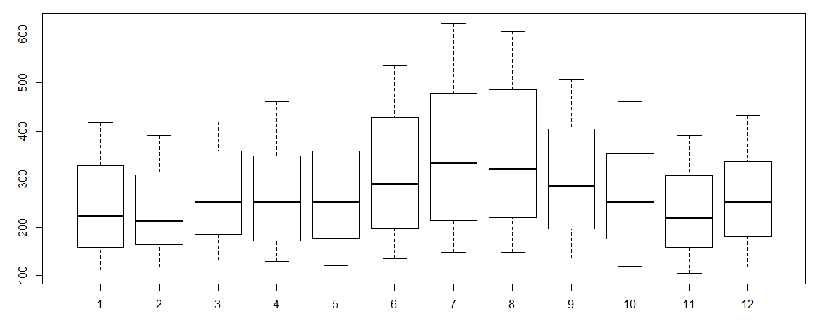
> boxplot(AirPassengers~cycle(AirPassengers))

#Box plot across months will give us a sense on seasonal effect

A few Inferences

1. The year on year trend clearly shows that the #passengers have been increasing without fail.
2. The variance and the mean value in July and August is much higher than rest of the months.
3. Even though the mean value of each month is quite different their variance is small. Hence, we have strong seasonal effect with a cycle of 12 months or less.

End Notes

Exploring data becomes most important in a time series model – without this exploration, you will not know whether a series is stationary or not. As in this case we already know many details about the kind of model we are looking out for. In next article we will take up a few time series models and their characterstics. In coming articles we will also take this problem forward and make a few predictions.

Did you find the article useful? Share with us if you have done similar kind of analysis before. Do let us know your thoughts about this article in the box below.

If you like what you just read & want to continue your analytics learning, subscribe to our emails, follow us on twitter or like our facebook page.

Tavish