Step by Step guide to learn Time Series Modeling

Introduction

Regression Models, both linear and logistic are an inevitable part of Analytics industry. Take a flashback & recall, when did you built your last Time Series model. Time series models are very useful models when you have serially correlated data. In case you have never built a time series model or you struggle with some concepts of time series models, you have landed at the right page.

Want to learn these concepts faster? Feel free to ask us your subject related queries & doubts here.

Learning Strategy

The next series of articles will help you to revise some basic concepts of Time Series. We will start with basic concepts like stationary series & random walk. Then, we’ll proceed to complex concepts like Seasonal ARIMA models.

Here is my initial thought for the series of articles:-

1. Stationary series and Random walk
2. Understanding time series models with an example
3. Auto-Regression and Moving Averages & Correlation Charts
4. ARIMA model (with or without seasonality adjustment)
5. Solving an ARIMA model on R

Stationary Series

There are three basic criterion for a series to be classified as stationary series :

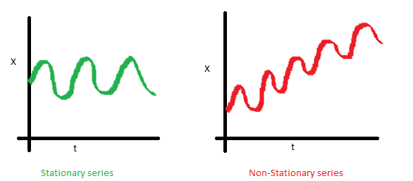
1. The mean of the series should not be a function of time rather should be a constant. The image below has the left hand graph satisfying the condition whereas the graph in red has a time dependent mean.

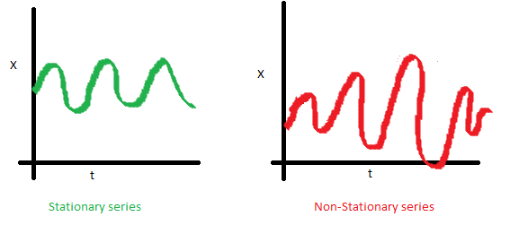
2. The variance of the series should not a be a function of time. This property is known as homoscedasticity. Following graph depicts what is and what is not a stationary series. (Notice the varying spread of distribution in the right hand graph)

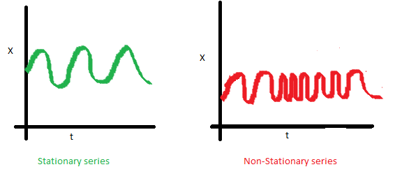
3. The covariance of the i th term and the (i + m) th term should not be a function of time. In the following graph, you will notice the spread becomes closer as the time increases. Hence, the covariance is not constant with time for the ‘red series’.

ALSO SEE: Brush up your basics. How to understand population distributions?

Why do I care about stationarity of a time series?

The reason I took up this section first was that until unless your time series is stationary, you cannot build a time series model. In cases where the stationary criterion are violated, the first requisite becomes to stationarize the time series and then try stochastic models to predict this time series. The are multiple ways of bringing this stationarity. Some of them are Detrending, Differencing etc.

Random Walk

This is the most basic concept of the time series. You might know the concept well. But, I found many people in the industry who interprets random walk as a stationary process. In this section with the help of some mathematics, I will make this concept crystal clear for ever. Let’s take an example.

Example: Imagine a girl moving randomly on a giant chess board. In this case, next position of the girl is only dependent on the last position.

(Source: http://scifun.chem.wisc.edu/WOP/RandomWalk.html )

Now imagine, you are sitting in another room and are not able to see the girl. You want to predict the position of the girl with time. How accurate will you be? Of course you will become more and more inaccurate as the position of the girl changes. At t=0 you exactly know where the girl is. Next time, she can only move to 8 squares and hence your probability dips to 1/8 instead of 1 and it keeps on going down. Now let’s try to formulate this series :

X(t) = X(t-1) + Er(t)

where Er(t) is the error at time point t. This is the randomness the girl brings at every point in time.

Now, if we recursively fit in all the Xs, we will finally end up to the following equation :

X(t) = X(0) + Sum(Er(1),Er(2),Er(3).....Er(t))

Now, lets try validating our assumptions of stationary series on this random walk formulation:

1. Is the Mean constant ?

E[X(t)] = E[X(0)] + Sum(E[Er(1)],E[Er(2)],E[Er(3)].....E[Er(t)])

We know that Expecation of any Error will be zero as it is random.

Hence we get E[X(t)] = E[X(0)] = Constant.

2. Is the Variance constant?

Var[X(t)] = Var[X(0)] + Sum(Var[Er(1)],Var[Er(2)],Var[Er(3)].....Var[Er(t)])

Var[X(t)] = t * Var(Error) = Time dependent.

Hence, we infer that the random walk is not a stationary process as it has a time variant variance. Also, if we check the covariance, we see that too is dependent on time.

Let’s spice up things a bit,

We already know that a random walk is a non-stationary process. Let us introduce a new coefficient in the equation to see if we can make the formulation stationary.

Introduced coefficient : Rho

X(t) = Rho * X(t-1) + Er(t)

Now, we will vary the value of Rho to see if we can make the series stationary. Here we will interpret the scatter visually and not do any test to check stationarity.

Let’s start with a perfectly stationary series with Rho = 0 . Here is the plot for the time series :

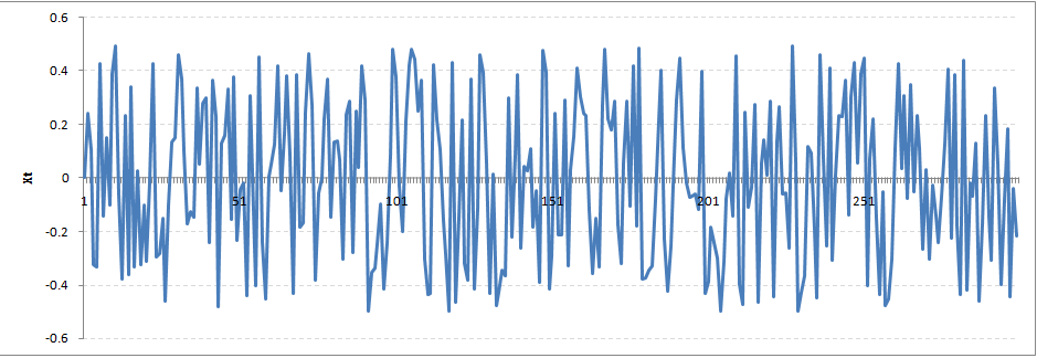
Increase the value of Rho to 0.5 gives us following graph :

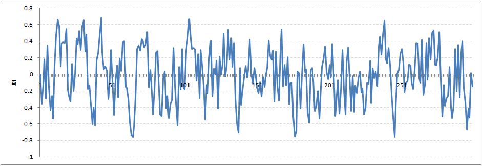
You might notice that our cycles have become broader but essentially there does not seem to be a serious violation of stationary assumptions. Let’s now take a more extreme case of Rho = 0.9

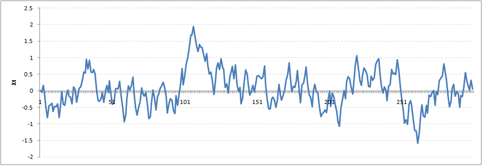
We still see that the X returns back from extreme values to zero after some intervals. This series also is not violating non-stationarity significantly. Now, let’s take a look at the random walk with rho = 1.

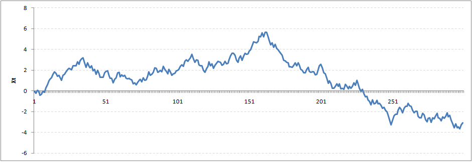
This obviously is an violation to stationary conditions. What makes rho = 1 a special case which comes out badly in stationary test? We will find the mathematical reason to this.

Let’s take expectation on each side of the equation  “X(t) = Rho * X(t-1) + Er(t)”

E[X(t)] = Rho *E[ X(t-1)]

This equation is very insightful. The next X (or at time point t) is being pulled down to Rho * Last value of X.

For instance, if X(t – 1 ) = 1, E[X(t)] = 0.5 ( for Rho = 0.5) . Now, if X moves to any direction from zero, it is pulled back to zero in next step. The only component which can drive it even further is the error term. Error term is equally probable to go in either direction. What happens when the Rho becomes 1? No force can pull the X down in the next step.

Dickey Fuller test of stationarity

What you just learnt in the last section is formally known as Dickey Fuller test. Here is a small tweak which is made for our equation to convert it to a Dickey Fuller test:

X(t) = Rho * X(t-1) + Er(t)

=>  X(t) - X(t-1) = (Rho - 1) X(t - 1) + Er(t)

We have to test if Rho – 1 is significantly different than zero or not. If the null hypothesis gets rejected, we’ll get a stationary time series.

End Notes

Stationary testing and converting a series into a stationary series are the most critical processes in a time series modelling. You need to memorize each and every detail of this concept to move on to the next step of time series modelling. In the next article, we will consider an example to show you how a time series looks like. Stay Tuned!

Did you find the article useful? Have you used time series modelling before? Share with us any such experiences. Do let us know your thoughts about this article in the box below.

If you like what you just read & want to continue your analytics learning, subscribe to our emails, follow us on twitter or like our facebook page.

Tavish